Introduction to Machine Learning

Original Source: https://www.coursera.org/learn/machine-learning

What is Machine Learning?

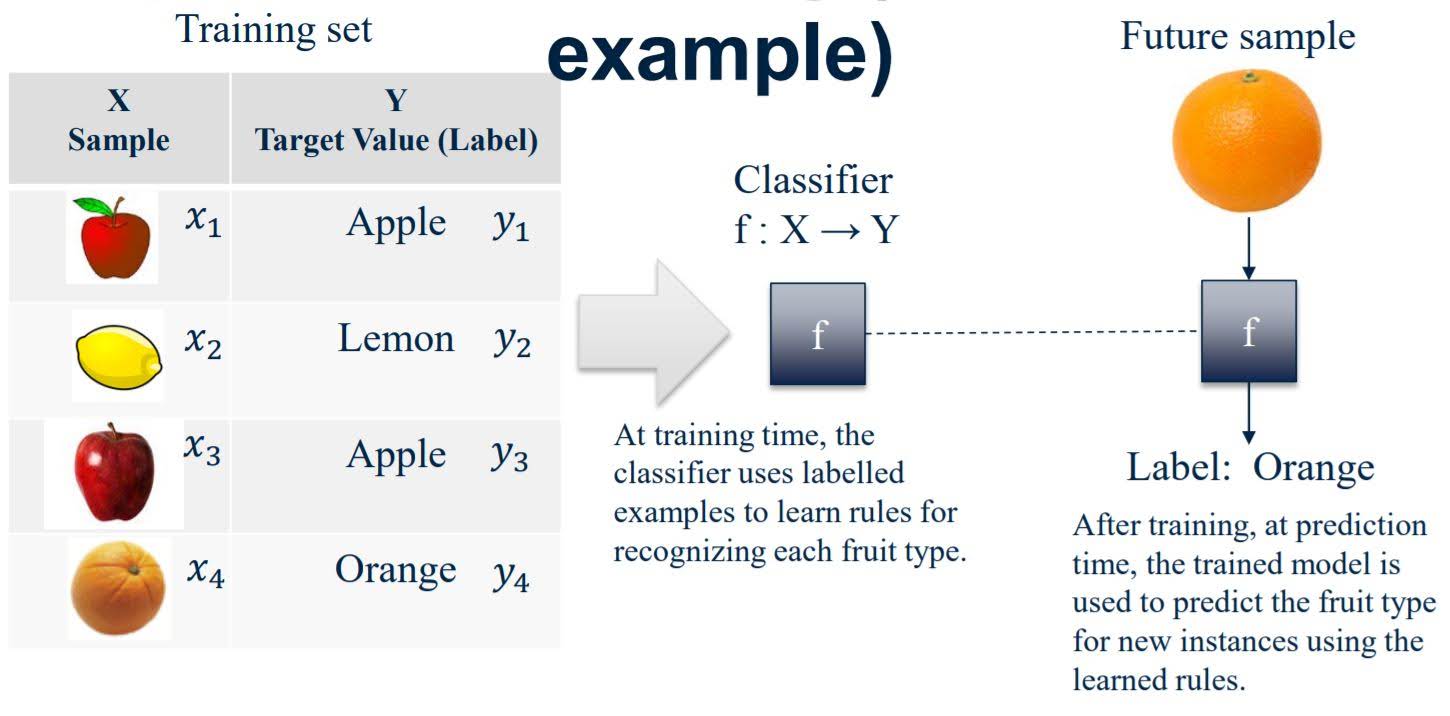
The study of computer programs (algorithms) that can learn by example

ML Algorithms learn rules from labelled examples.

• A set of labelled examples used for learning is called training data.
• The learned rules should also be able to generalize to correctly recognize or predict new examples not in the training set.

Machine Learning brings together statistics, computer science, and more, depending on the specific goal.

Examples of Machine Learning

• Fraud detection
  Training Data: Credit card transaction history
  Label: Whether each transaction was fraud.
  Develop model that predicts which transactions are fraudulent.
• Web search: query spell-checking, result ranking, content classification and selection, advertising placement.
• Speech Recognition
• eCommerce: Product recommendations
• Email spam filtering
• Health applications: Drup design and discovery
• Education: Automated essay scoring

Categories of Machine Learning

A. Supervised machine learning

Model learns to predict target values from labelled data. The example ‘Fraud detection’ above is a supervised classification machine learning task.

1. Classification

Target values are discrete classes

2. Regression

Target values are continuous values

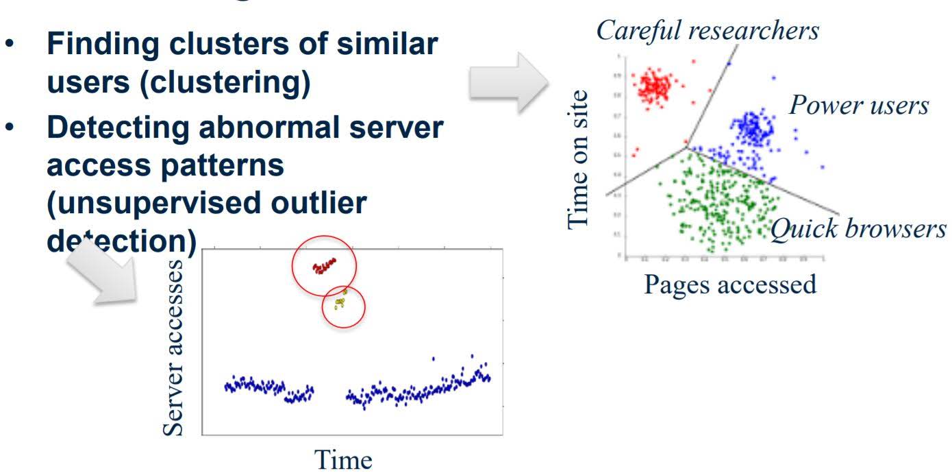
B. Unsupervised machine learning

Find structure in unlabeled data

1. Clustering
   ex) Finding clusters of similar users
2. Unsupervised outlier detection
   ex) Detecting abnormal server access patterns

Basic Machine Learning Workflow

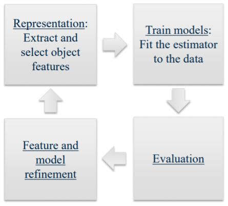
1. Representation

Extract and select object features

2. Train models

Fit the estimator to the data

3. Evaluation

Does this feature and estimator predict successfully?

4. Feature and model refinement

Python Tools for Machine Learning

1. scikit-learn: Python Machine Learning Library
2. NumPy: Scientific computing library
3. Pandas: Data manipulation
4. matplotlib: plotting library

k-Nearest Neighbor (k-NN) Classifier

1. Find the most similar instances (let’s call them X_NN) to x_test that are in X_train.
2. Get the labels y_NN for the instances in X_NN
3. Predict the label for x_test by combining the labels y_NN (e.g. simple majority vote)

k-NN needs four things specified

1. A distance metric
   Typically Euclidean (Minkowski with p = 2)
2. How many ‘nearest’ neighbors to look at?
   e.g. five
3. Optional weighting function on the neighbor points
   Typically ignored
4. How to aggregate the classes of neighbor points
   Typically Simple majority vote (Class with the most representatives among nearest neighbors)

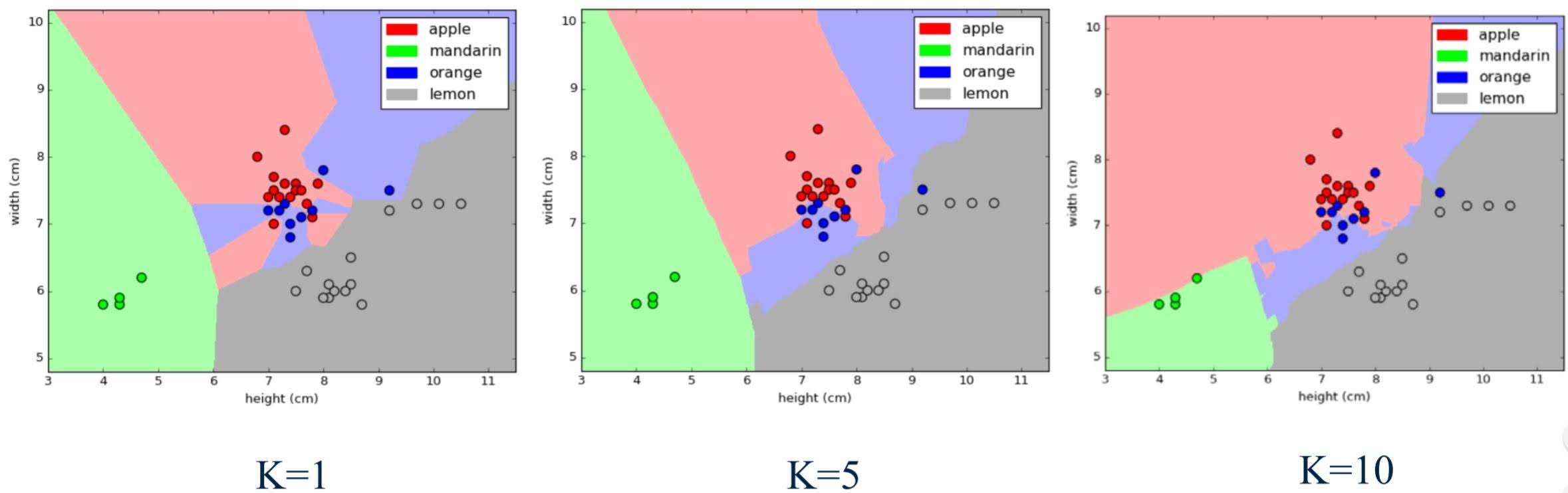
Visual explaining effect of ‘k’

Example Machine Learning Problem with k-NN

Import required modules and load data file

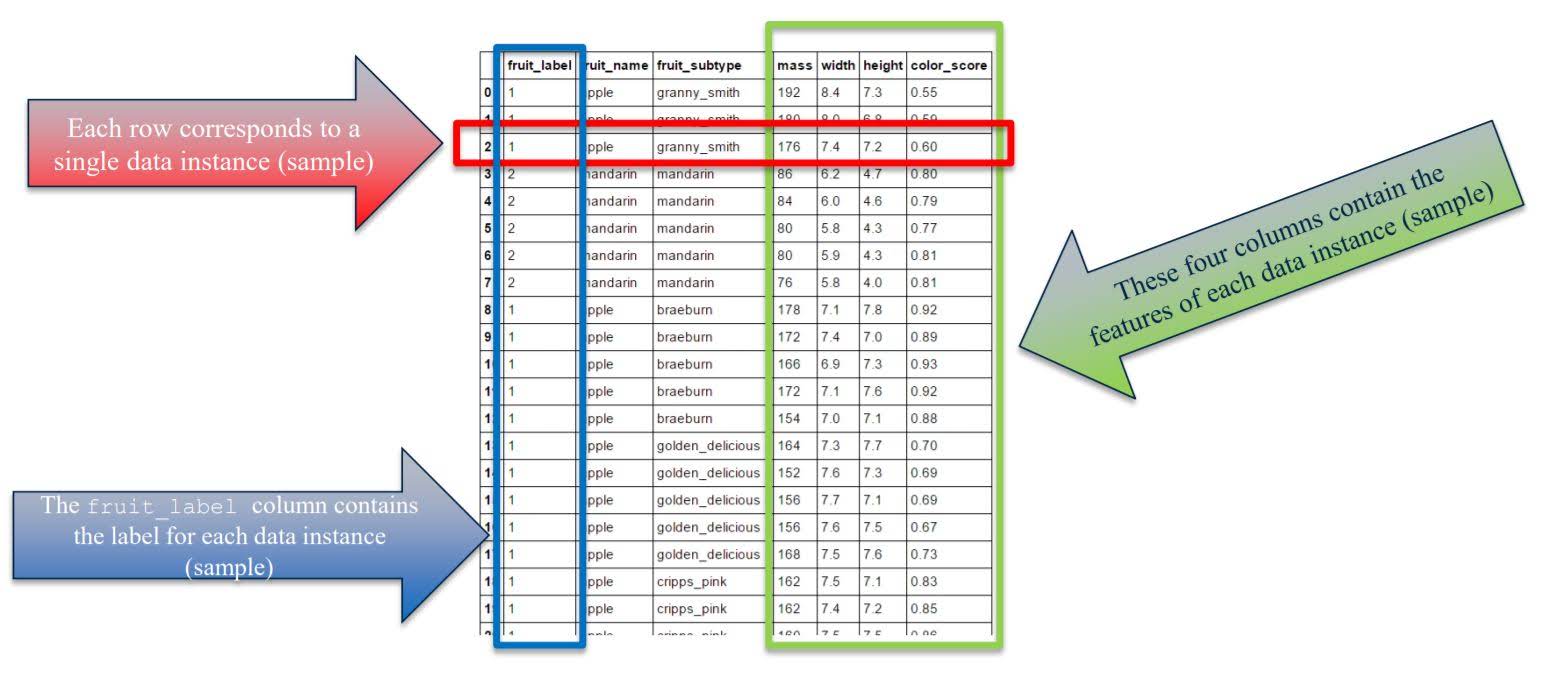
The input data as a table

%matplotlib inline

import numpy as np
import matplotlib.pyplot as plt
import pandas as pd
from sklearn.model_selection import train_test_split

# set default figure size to (14, 8)
plt.rcParams['figure.figsize'] = (14.0, 8.0)

fruits = pd.read_table('fruit_data_with_colors.txt')

fruits.shape

(59, 7)

fruits.head()

	fruit_label	fruit_name	fruit_subtype	mass	width	height	color_score
0	1	apple	granny_smith	192	8.4	7.3	0.55
1	1	apple	granny_smith	180	8.0	6.8	0.59
2	1	apple	granny_smith	176	7.4	7.2	0.60
3	2	mandarin	mandarin	86	6.2	4.7	0.80
4	2	mandarin	mandarin	84	6.0	4.6	0.79

# create a mapping from fruit label value to fruit name to make results easier to interpret
lookup_fruit_name = dict(zip(fruits.fruit_label.unique(), fruits.fruit_name.unique()))   
lookup_fruit_name

{1: 'apple', 2: 'mandarin', 3: 'orange', 4: 'lemon'}

Create train-test split

If we use whole data as training set, our model can overfit to training set so it might not generalize to real world cases. Thus, we evaluate our model with hold-out validation set or development set and tune our hyperparmeters(e.g. value k in k-NN) based this evaluation.
sklearn.model_selection.train_test_split splits data into train set and test(validation, development) set.

# For this example, we use the mass, width, and height features of each fruit instance
X = fruits[['mass', 'width', 'height', 'color_score']]
y = fruits['fruit_label']

# default is 75% / 25% train-test split
X_train, X_test, y_train, y_test = train_test_split(X, y, random_state=0)

print(X_train.shape)
print(X_test.shape)
print(y_train.shape)
print(y_test.shape)

(44, 4)
(15, 4)
(44,)
(15,)

Examining the data

Reasons why looking at the data initially is important

• Inspecting feature values may help identify what cleaning or preprocessing still needs to be done once you can see the range or distribution of values that is typical for each attribute.
• You might notice missing or noisy data, or inconsistencies such as the wrong data type being used for a column, incorrect units of measurements for a particular column, or that there aren’t enough examples of a particular class.
• You may realize that your problem is actually solvable without machine learning.

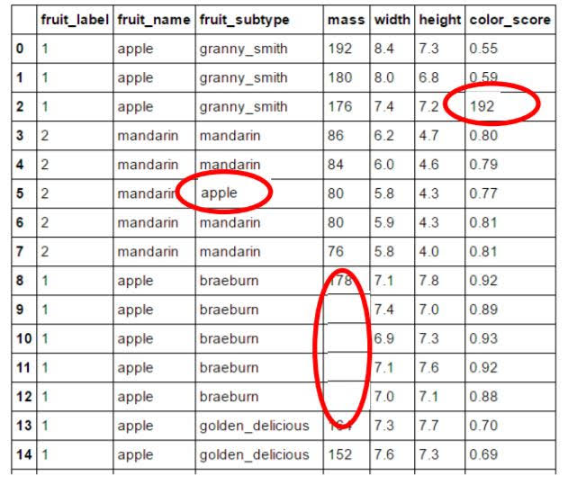
Example of incorrect or missing feature values

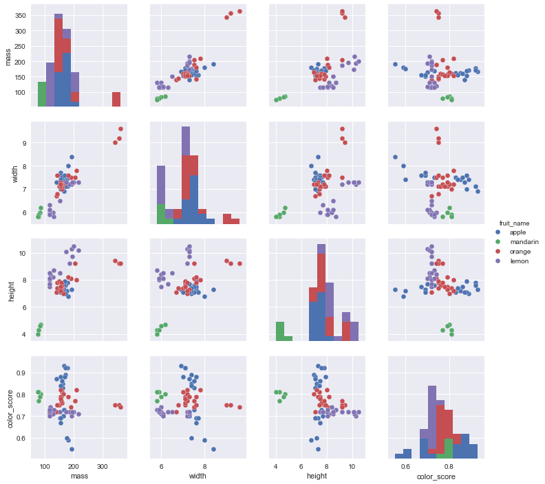
Plotting pairwise feature scatterplot
It visualizes the data using all possible pairs of features, with one scatterplot per feature pair, and histograms for each feature along the diagonal.

import seaborn as sns
sns.set()
sns.pairplot(fruits.iloc[:, 1:], hue='fruit_name')

<seaborn.axisgrid.PairGrid at 0x179d2a53748>

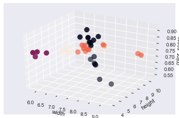
A three-dimensional feature scatterplot

# plotting a 3D scatter plot
from mpl_toolkits.mplot3d import Axes3D

fig = plt.figure()
ax = fig.add_subplot(111, projection = '3d')
ax.scatter(X_train['width'], X_train['height'], X_train['color_score'], c = y_train, marker = 'o', s=100)
ax.set_xlabel('width')
ax.set_ylabel('height')

ax.set_zlabel('color_score')
plt.show()

Create classifier object

from sklearn.neighbors import KNeighborsClassifier

knn = KNeighborsClassifier(n_neighbors = 5)

Train the classifier (fit the estimator) using the training data

knn.fit(X_train, y_train)

KNeighborsClassifier(algorithm='auto', leaf_size=30, metric='minkowski',
           metric_params=None, n_jobs=1, n_neighbors=5, p=2,
           weights='uniform')

Estimate the accuracy of the classifier on future data, using the test data

knn.score(X_test, y_test)

0.5333333333333333

Use the trained k-NN classifier model to classify new, previously unseen objects

# first example: a small fruit with mass 20g, width 4.3 cm, height 5.5 cm
fruit_prediction = knn.predict([[20, 4.3, 5.5, 0.5]])
lookup_fruit_name[fruit_prediction[0]]

'mandarin'

# second example: a larger, elongated fruit with mass 100g, width 6.3 cm, height 8.5 cm
fruit_prediction = knn.predict([[100, 6.3, 8.5, 0.5]])
lookup_fruit_name[fruit_prediction[0]]

'lemon'

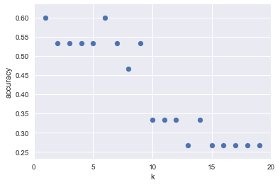
How sensitive is k-NN classification accuracy to the choice of the ‘k’ parameter?

k_range = range(1,20)
scores = []

for k in k_range:
    knn = KNeighborsClassifier(n_neighbors = k)
    knn.fit(X_train, y_train)
    scores.append(knn.score(X_test, y_test))

plt.figure()
plt.xlabel('k')
plt.ylabel('accuracy')
plt.scatter(k_range, scores)
plt.xticks([0,5,10,15,20])
plt.show()