Supervised Learning

Original Source: https://www.coursera.org/learn/machine-learning

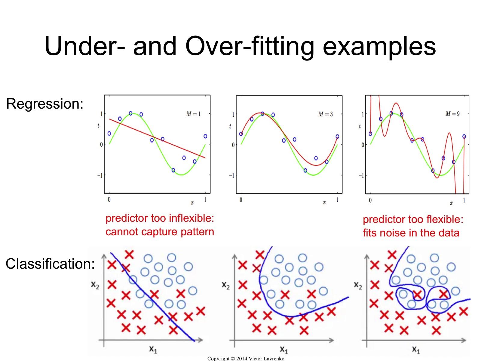
Overfitting and Underfitting

Generalization ability refers to an algorithm’s ability to give accurate predictions for new, previously unseen data.

Models that are too complex for the amount of training data available are said to overfit and are not likely to generalize well to new examples.

Models that are too simple, that don’t even do well on the training data, are said to underfit and also not likely to generalize well.

To solve this problem, we split our data into training set and validation set. Then we train our model on training set and evaluate our trained model with validation set. We tune our hyperparamters and do this again, until we find good model with good hyperparameters.

One method to prevent overfitting is regularization. Regularization makes weights decrease, thus simplifies the model.

The relationship between model complexity and training/test performance

Cross-validation

We splitted data into train set and validation set, trained the model on train set and evaluated on the validation set.

However, the accuracy score of a supervised learning method can vary, depending on which samples happen to end up in the training set.

So we will now use multiple train-test splits, not just a single one.
Results are averaged over multiple different training sets instead of relying on a single model trained on a particular training set.

5-fold cross-validation example

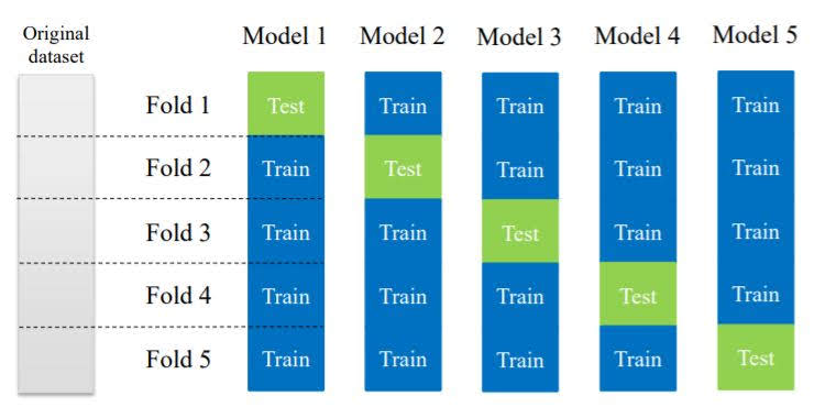
To maintain class proportions of the total dataset even after splitting, we use stratified cross-validation.

Stratified folds each contain a proportion of classes that matches the overall dataset.

Evaluation Metrics

It’s very important to choose evaluation methods that match the goal of your application.

Regression

R-squared regression score (coefficient of determination)

The score is between 0 and 1.
A value of 0 corresponds to a constant model that predicts the mean value of all training target values, and a value of 1 corresponds to perfect prediction.

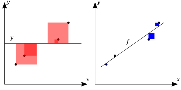
$R^{2}=1-{\frac {\color {blue}{SS_{\text{res}}}}{\color {red}{SS_{\text{tot}}}}}$

Classification

Accuracy

The ratio of correct predictions of all predictions.

Precision & Recall

With imbalanced classes, accuracy is not an effective metric. For example, predicting that a patient doesn’t have cancer will yield accuracy of almost 100%.

To solve this problem, we use evaluation metric ‘Precision’, ‘Recall’ and ‘F1-Score’ that combine two together.

Confusion matrix for binary prediction task

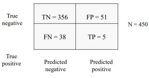
Precision(Positive Predictive Value): What fraction of positive predictions are correct? \({\displaystyle \mathrm {PPV} ={\frac {\mathrm {TP} }{\mathrm {TP} +\mathrm {FP} }}}\)

Recall(True Positive Rate): What fraction of all postitive instances does the classifier correctly identify as positive? \({\displaystyle \mathrm {TPR} ={\frac {\mathrm {TP} }{\mathrm {TP} +\mathrm {FN} }}}\)

F1 Score: harmonic mean of precision and recall \({\displaystyle F_{1}=2\cdot {\frac {\mathrm {PPV} \cdot \mathrm {TPR} }{\mathrm {PPV} +\mathrm {TPR} }}={\frac {2\mathrm {TP} }{2\mathrm {TP} +\mathrm {FP} +\mathrm {FN} }}}\)

Multiclass Classification

In a n-class classification, there are n precision scores, one for each class. There are two ways to average this to yield one evaluation metric.

1. Macro-average: Each class has equal weight.
   1. Compute metric within each class
   2. Average resulting metrics across classes
2. Micro-average: Each instance has equal weight, so largest classes have most influence.
   1. Aggregrate outcomes across all classes
   2. Compute metric with aggregate outcomes

Example

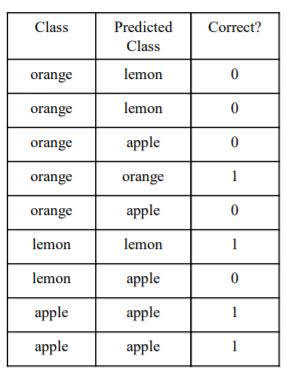
Macro-average: (1/5(orange) + 1/2(lemon) + 2/2(apple))/3 = 0.57
Micro-average: 4/9 = 0.44

If you want to weight your metric toward the largest ones, use micro-averaging.
If you want to weight your metric toward the smallest ones, use macro-averaging

Tradeoff between precision and recall

There is often a tradeoff between precision and recall, and here’s a way to emphasize one of them.

For each instance, a classifier applies decision functions and yields decision score. Then decides a decision threshold, and assign all instances that have decision score larger than decision threshold as 1 and all the others as 0.

Similarly, for each instance, a classifier yields probability score of class membership. The default probability threshold 0.5. If the instance’s probability score is larger than probability threshold, that instance will be assigned 1, and others will be assigned 0.

If we increase decision threshold or probability threshold, precision will go high and recall low.
If we decrease decision threshold or probability threshold, precision will go down an recall will go up.

ROC AUC Score

ROC Curve

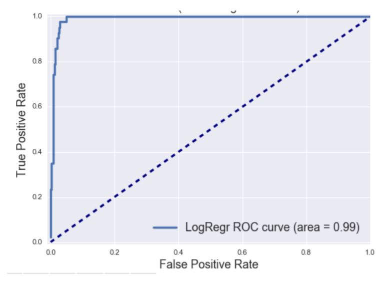
Top left corner is the ideal point.

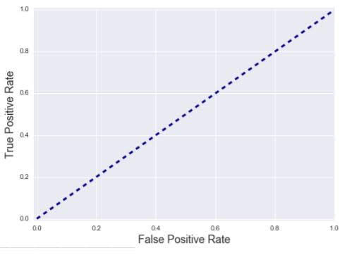
Random guessing

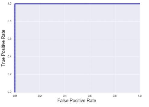
Perfect classifier

ROC AUC is the total area under the ROC curve.
AUC=0: worst classifier
AUC=1: best classifier

In scikit-learn, roc_auc_score is not defined in multiclass classification. Also, you need to pass trained_model.predict_proba(X) as argument y_score to get results.

Feature Normalization

Important for some machine learning methods that all features are on the same scale (e.g. faster convergence in learning, more uniform or ‘fair’ influence for all weights)

Used in regularized regression, k-NN, support vector machines, neural networks, …

One example is ‘MinMax scaling’ of the features

For each feature, compute the min value and max value achieved across all instances in the training set.
Then for each feature, transform a given feature to a scaled version using the formula \(x'_i=\frac{x_i-x_i^{MIN}}{x_i^{MAX}-x_i^{MIN}}\)

Caution: The validation or test set must use identical scaling to the training set.

Data Leakage

When the data you’re using to train contains information about what you’re trying to predict, we call it ‘data leakage’. When data leakage happened the evaluation of that model becomes too optimistic.

Minimizing Data Leakage

• Perform data preparation within each cross-validation fold separately
  • Scale/normalize data, perform feature selection, etc. within each fold separately, not using the entire dataset.
  • For any such parameters estimated on the training data, you must use those same parameters to prepare data on the corresponding held-out test fold.
• With time series data, use a timestamp cutoff
  • The cutoff value is set to the specific time point where prediction is to occur using current and past records.
  • Using a cutoff time will make sure you aren’t accessing any data records that were gathered after the prediction time, i.e. in the future.
• Before any work with a new dataset, split off a final test validation dataset if you have enough data
  • Use this final test dataset as the very last step in your validation
  • Helps to check the true generalization performance of any trained models

K-Nearest Neighbors

Algorithm

Given a training set X_train with labels y_train, and given a new instance x_test to be classified

1. Find the most similar instances (let’s call them X_NN) to x_test that are in X_train.
2. Get the labels y_NN for the instances in X_NN
3. Predict the label for x_test by combining the labels y_NN (e.g. simple majority vote)

For Regression

For each point in unlabeled feature vector space, find k nearest neighbors of labeled data points. Assign average of those points’ label to that unlabeled point.

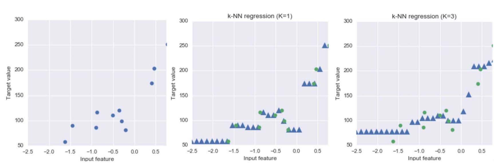
Hyperparmeters

• n_neighbors(k): number of neares neighbors to consider (Default 5)
• metric: distance function between data points (Default Euclidean)

Linear Algorithms

Linear Regression (for regression)

Find a line that best represents input feature vector instances.

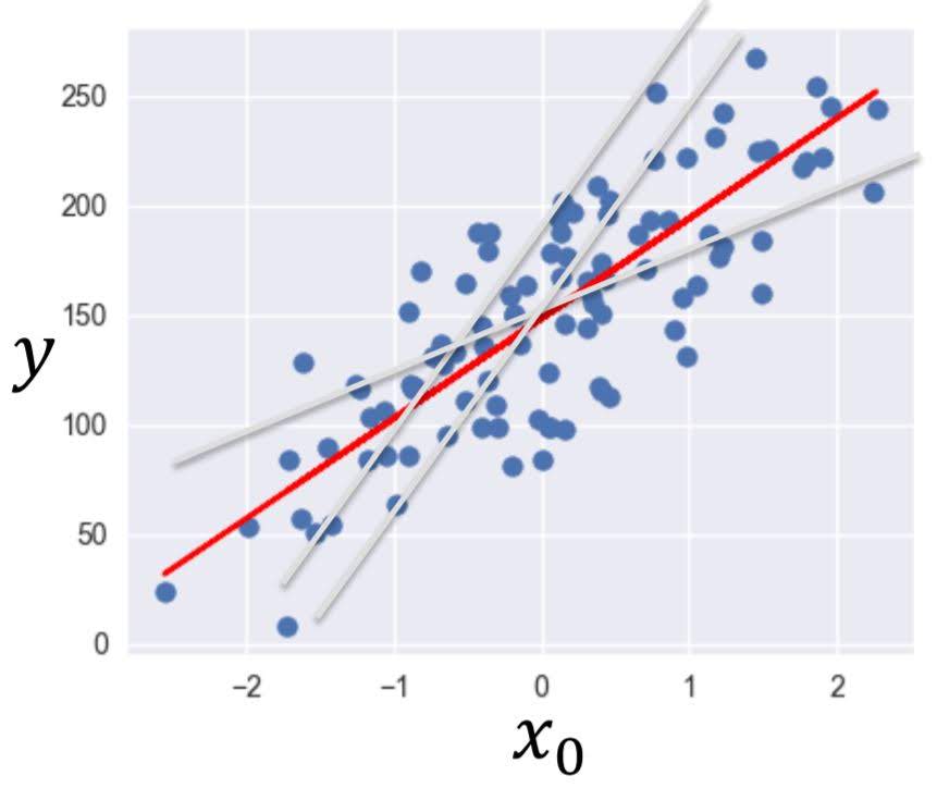
In the above image, red line best represents the data points. That is the result of linear regression.

• Input feature vector: $x=(x_0,x_1,…,x_n)$
• Predicted output: $\hat{y}=\hat{w_0}x_0+\hat{w_1}x_1+…+\hat{w_n}x_n+\hat{b}$
• Parameters to estimate
  • feature weights: $(\hat{w_o},…,\hat{w_n})$
  • bias term: $\hat{b}$

Specifically, find parameters that minimizes the cost function of the linear model, which is ‘sum squared error’ Sum squared error is the sum of squared differences between predicted target and actual target values. \(C(\textbf{w},b)=\sum_{i=1} (y_i-(\textbf{w}\textbf{x}_i+b))^2\)

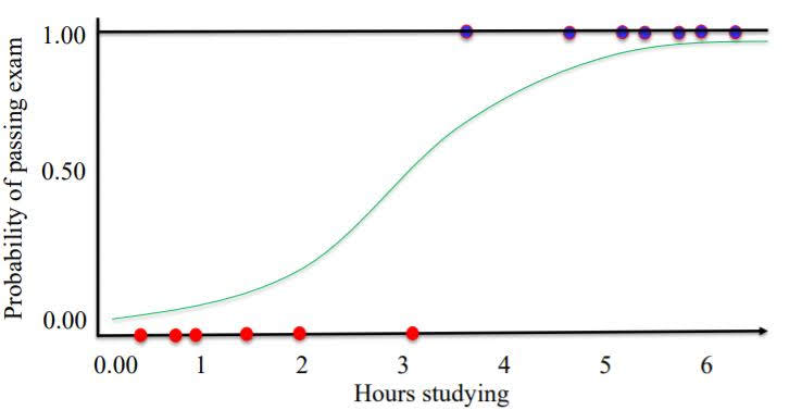
Logistic Regression (for classification)

It’s almost the same as linear regression explained above, but it has two differences.

First, the output of linear function is not a scalar value but a n-dimension vector, where n is the number of possible classes.

Second, ‘logistic function’ is applied to the output of linear function. The logistic function transforms real-valued input to an output number y between 0 and 1, interpreted as the probability the input object belongs to the positive class.

example of binary logistic regression with 1-dimensional feature vector.

Hyperparameters

• C: Larger values of C mean less regularization (Default 1)

Regularization

To prevent overfitting, we can add regularization to linear regression.

We will add regularization term to the cost function.

Ridge(L2) Regression

\[C(\textbf{w},b)=\sum_{i=1} (y_i-(\textbf{w}\textbf{x}_i+b))^2+\alpha \sum_{j=1}^p w_j^2\]

Lasso(L1) Regression

\[C(\textbf{w},b)=\sum_{i=1} (y_i-(\textbf{w}\textbf{x}_i+b))^2+\alpha \sum_{j=1}^p \|w_j\|\]

If feature weights w increases, cost will increase, so the process of minimizing cost will make w smaller, thus make the model simpler.

We use L2 Regression as default. L1 Regression has the effect of setting parameter weights in w to zero for the least influential variables. This is called a sparse solution.

Bigger $\alpha$ means more regularization. Default is 1.

Hyperparmeters

• alpha: weight given to the L1 or L2 regularization term in regression models (Default 1)

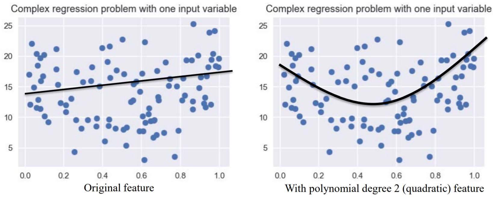
Linear Algorithm with Polynomial Features

Consider linear regression with two features $(x_0,x_1)$.
We will not generate new features consisting of all polynomial combinations of the original two features. That is, $(x_0,x_1,x_0^2, x_0x_1, x_1^2)$.
Then we do linear regression with these features.

Polynomial features can help build more complex models, but at the same time prone to overfitting.

Support Vector Machine

It is a classifier with maximum margin.

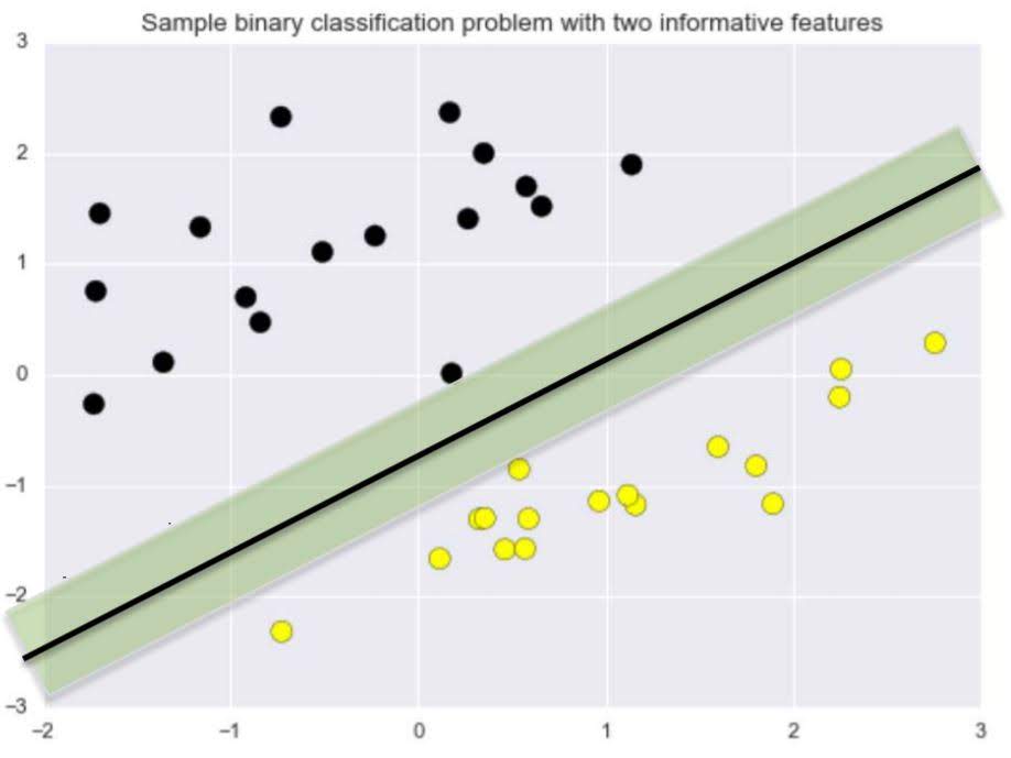
If the decision boundary(a boundary that seperates different classes in the feature space) is linear, it is called linear Support Vector Machine.

Kernelized Support Vector Machines

Before applying linear support vector machine, transform the original input space to make it much easier for a linear classifier.

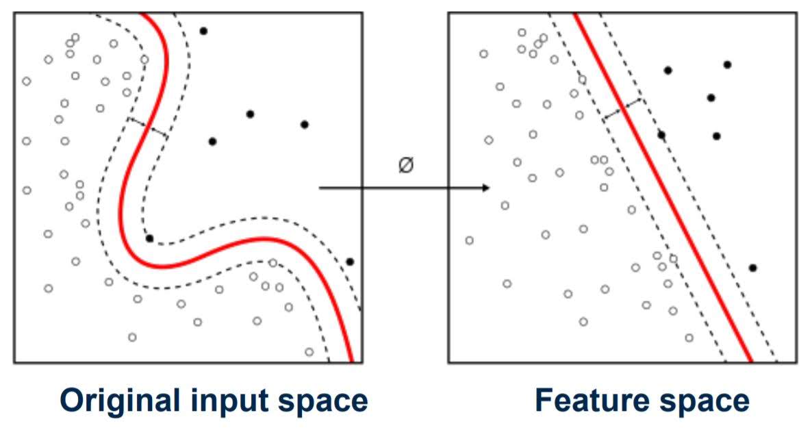
The most common kernel is Radial Basis Function Kernel (RBF Kernel).

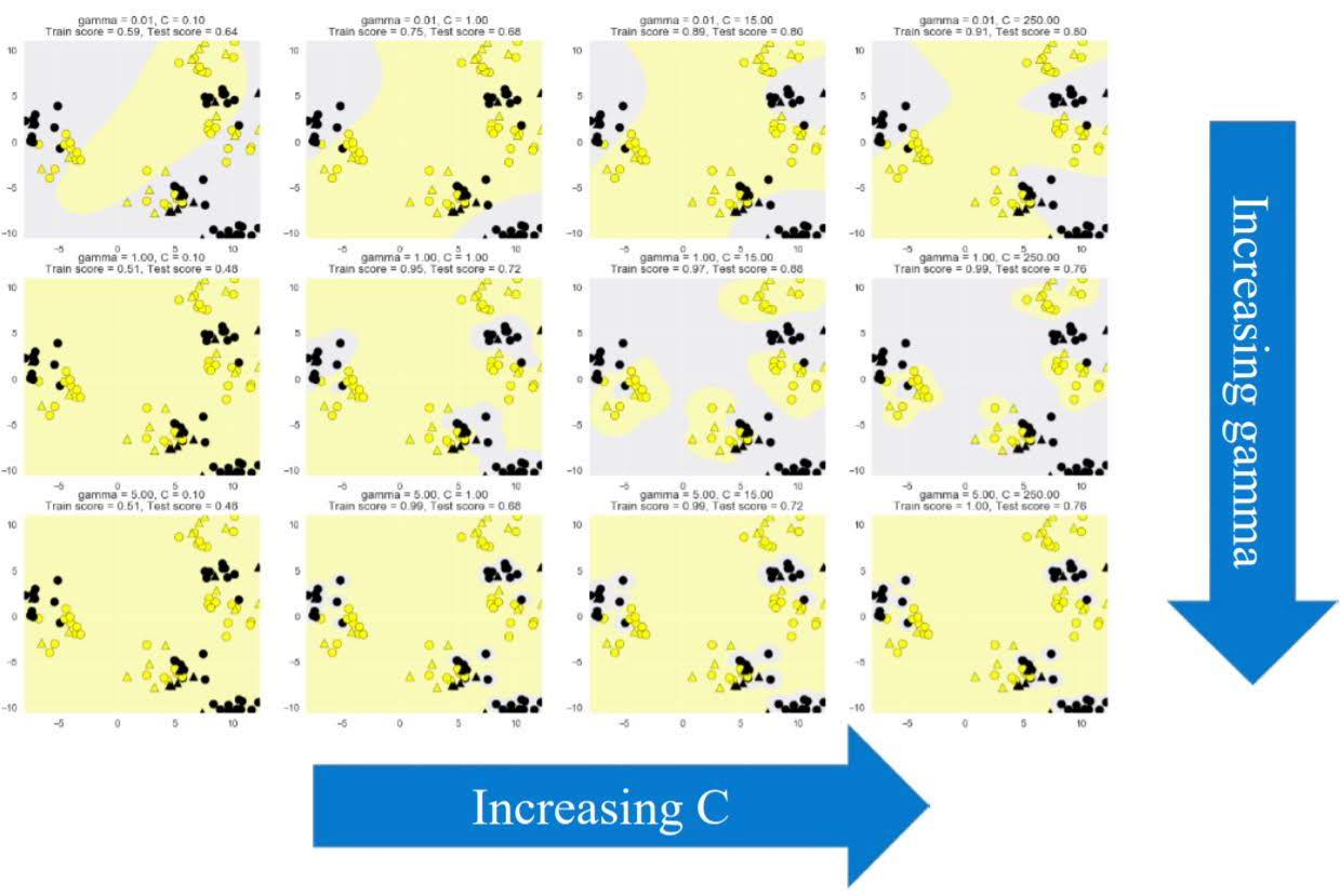
Hyperparmeters

• kernel: Type of kernel function to be used (Default ‘rbf’)
• gamma: RBF kernel width
• C: Larger values of C mean less regularization (Default 1)

The effect of RBF gamma parameter and C.

Decision Tree

Example

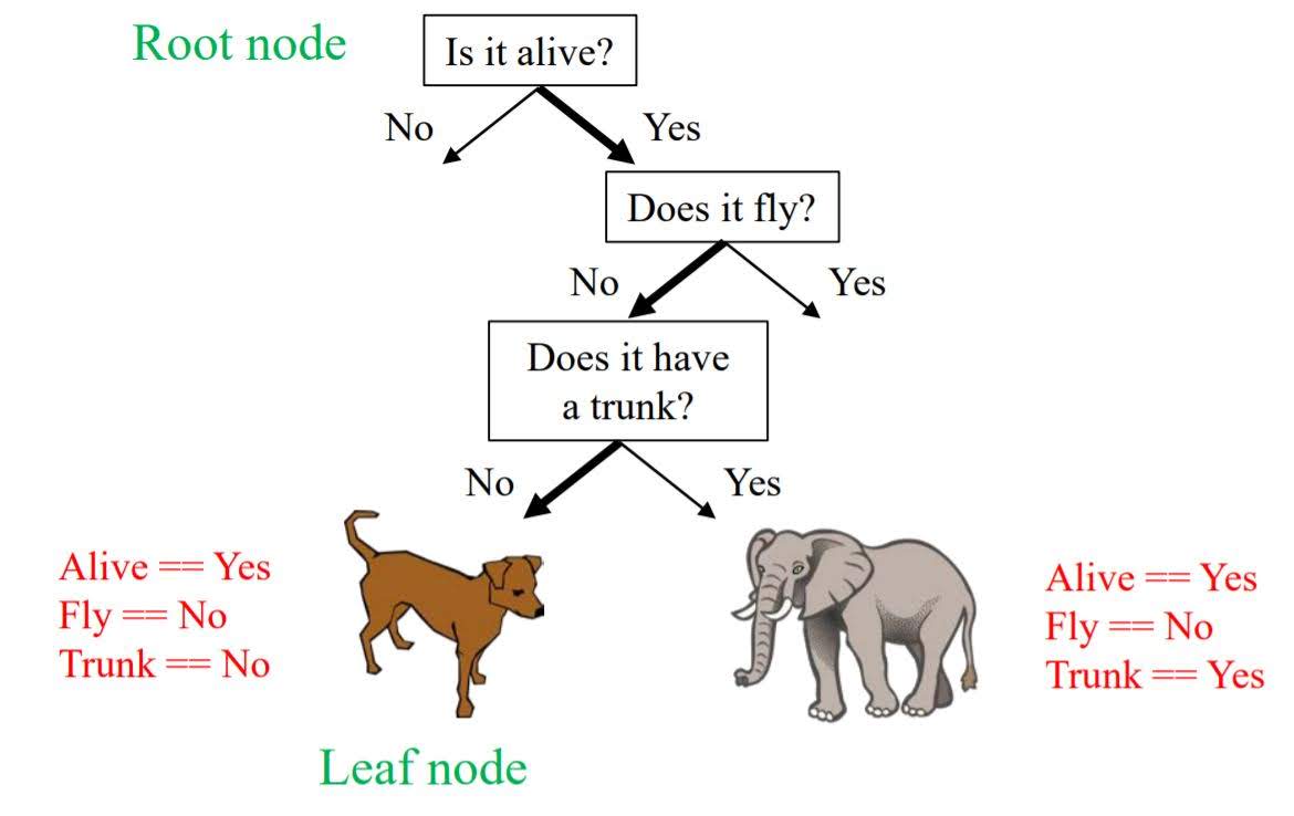
Decision trees are easily visualized and interpreted. It also works well with datasets using a mixture of feature types. However, it can often overfit so we usually need an ensemble of trees for better generalization performance.

Feature importance

How important is a feature to overall prediction accuracy?

• A number between 0 and 1 assigned to each feature.
• Feature importance of 0 the feature was not used in prediction.
• Feature importance of 1 the feature predicts the target perfectly.
• All feature importances are normalized to sum to 1.

Hyperparmeters

• max_depth: controls maximum depth (number of split points). Most common way to reduce tree complexity and overfitting.

Naive Bayes Classifier

These classifiers are called ‘Naive’ because they assume that features are conditionally independent, given the class.

It has a highly efficient learning and prediction, but generalization performance may worse than more sophisticated learning methods.

Types

• Bernoulli: binary features (e.g. word presence/absence)
• Multinomial: discrete features (e.g. word counts)
• Gaussian: continuous/real-valued features

Gaussian Naive Bayes Classifier

The Gaussian Naive Bayes Classifier assumes that the data for each class was generated by a simple class specific Gaussian distribution.

During training, the Gaussian Naive Bayes Classifier estimates for each feature the mean and standard deviation of the feature value for each class.

For prediction, the classifier compares the features of the example data point to be predicted with the feature statistics for each class and selects the class that best matches the data point.

Predicting the class of a new data point corresponds mathematically to estimating the probability that each classes Gaussian distribution was most likely to have generated the data point. Classifier then picks the class that has the highest probability.

---

Ensemble

An ensemble is just a collection of predictors which come together (e.g. mean of all predictions) to give a final prediction.

There are two types of ensembels; Bagging and Boosting

Bagging is a simple ensembling technique in which we build many independent predictors/models/learners and combine them using some model averaging techniques. (e.g. weighted average, majority vote or normal average)

Boosting is an ensemble technique in which the predictors are not made independently, but sequentially.

We will look two pupular algorithms of ensemble here; Random Foreset which uses bagging and Gradient Boosted Decision Trees which uses boosting.

Random Forest

An ensemble of decision trees.

One decision tree was prone to overfitting. Ensemble of decision trees is more stable and generalize well.
It is widely used and yield very good results on many problems.

Algorithm

Each tree is grown as follows:

1. Each tree were built from a different random sample of the data called the bootstrap sample. If your training set has N instances or samples in total, a bootstrap sample of size N is created by just repeatedly picking one of the N dataset rows at random with replacement, that is, allowing for the possibility of picking the same row again at each selection. This sample will be the training set for growing the tree.
2. If there are M input features, a number m«M is specified such that at each node, m features are selected at random out of the M and the best split on these m is used to split the node. The value of m is held constant during the forest growing.

Then, combine individual predictions of each tree.

• Regression: mean of individual tree predictions.
• Classification:
  • Each tree gives probability for each class.
  • Probabilities averaged across trees.
  • Predict the class with highest probability

Hyperparameters

• n_estimators: number of trees to use in ensemble (default: 10).
• max_features: has a strong effect on performance. Influences the diversity of trees in the forest. (Default works well in practice)
• max_depth: controls the depth of each tree (default: None. Splits until all leaves are pure).

Gradient Boosted Decision Trees

Unlike the random forest method that builds and combines a forest of randomly different trees in parallel, the key idea of gradient boosted decision trees is that they build a series of trees. Where each tree is trained, so that it attempts to correct the mistakes of the previous tree in the series.

Hyperparameters

• n_estimators: sets # of small decision trees to use (weak learners) in the ensemble.
• learning_rate: The learning rate controls how hard each new tree tries to correct remaining mistakes from previous round.
  • High learning rate: more complex trees
  • Low learning rate: simpler trees
• n_estimators: adjusted first, to best exploit memory and CPUs during training, then other parameters.
• max_depth: typically set to a small value (e.g. 3-5) for most applications.

Neural Network

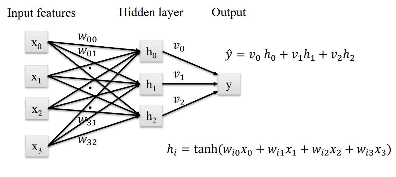
It’s basically linear regression or logistic regression with hidden layers.

In hidden layers, we apply activation function to add nonlinearity. Default activation function is ‘relu’.

More units in hidden layer and more hidden layers make model more complex.

Neural Networks with many hidden layers are called ‘Deep Learning’ architectures.

Hyperparameters

• hidden_layer_sizes: sets the number of hidden layers (number of elements in list), and number of hidden units per layer (each list element). (Default: 100)
• alpha: controls weight on the regularization penalty that shrinks weights to zero. (Default: alpha = 0.0001)
• activation: controls the nonlinear function used for the activation function, including: ‘relu’ (default), ‘logistic’, ‘tanh’.