Intro to Networks and Basics on NetworkX

Original Source: https://www.coursera.org/specializations/data-science-python

Introduction to Networks

What is networks?

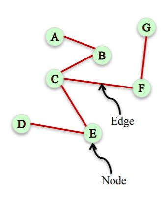
A set of objects (nodes) with interconnections (edge)
A representation of connections among a set of items

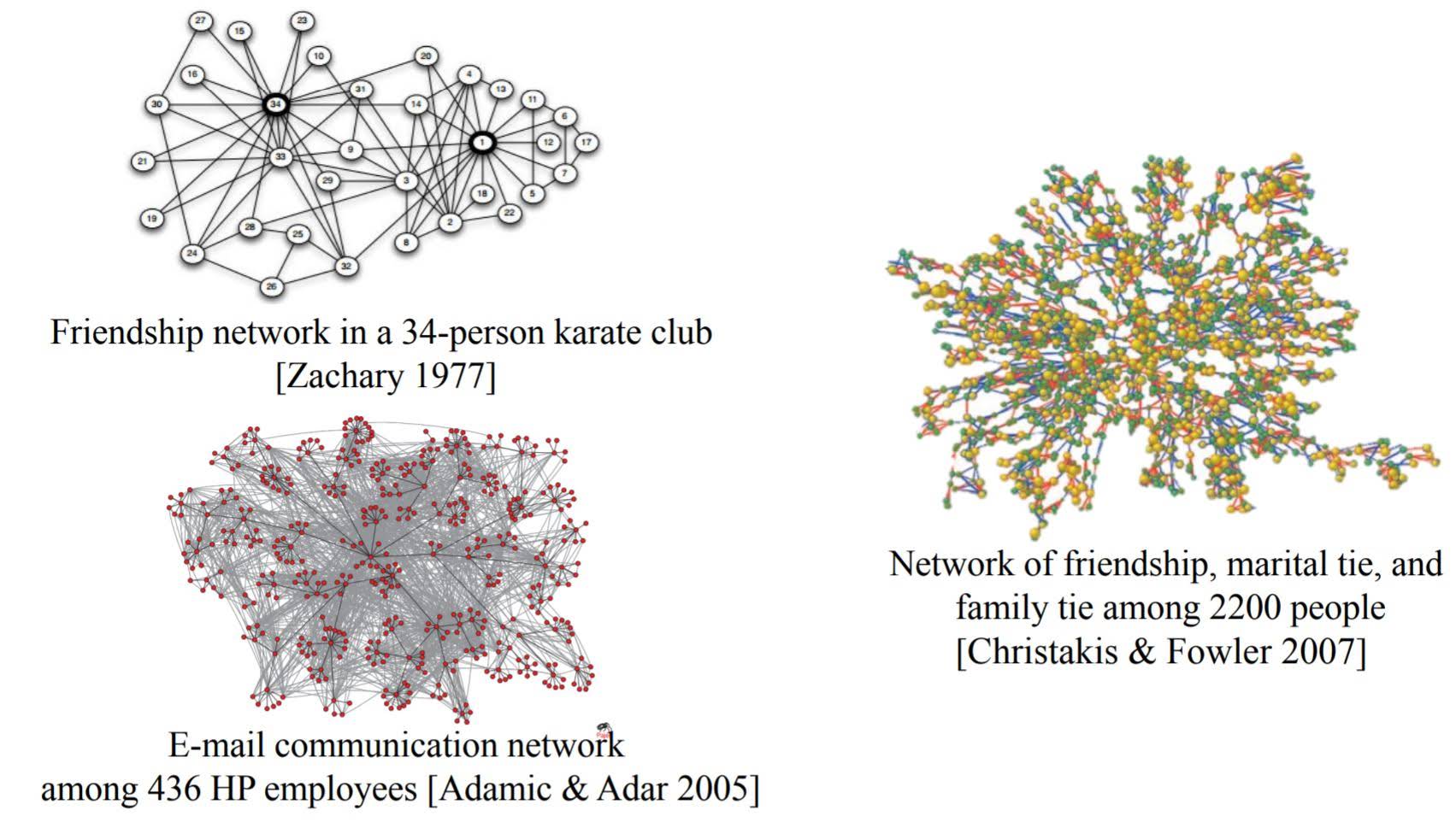
Examples of networks

• Social Networks
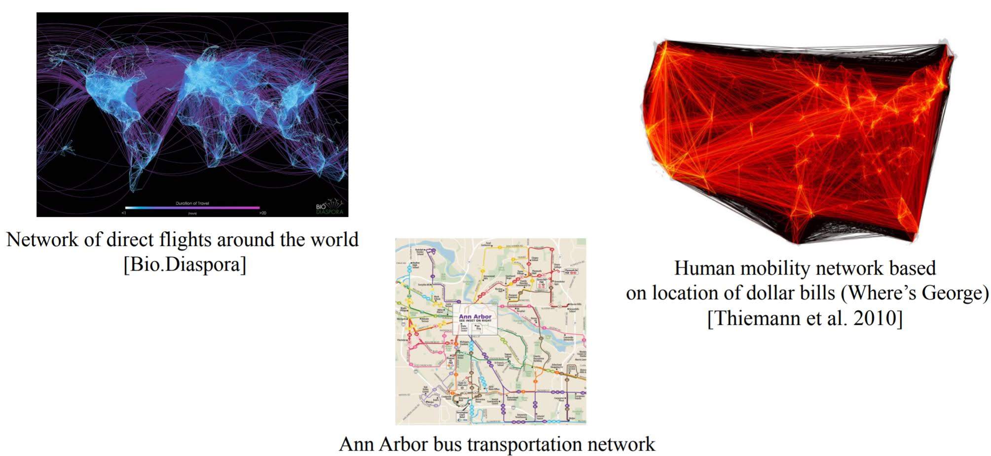
• Transportation and Mobility Networks
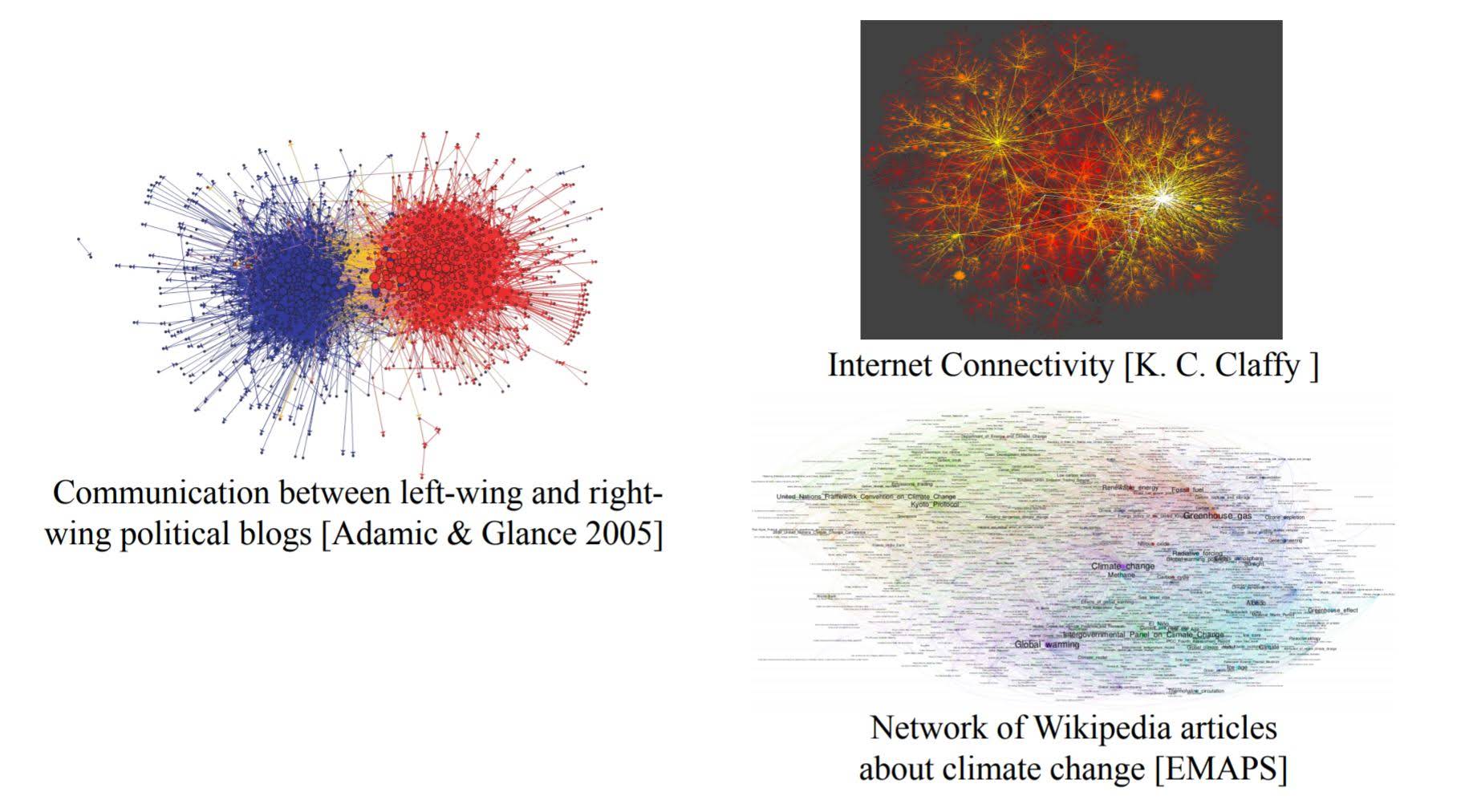
• Information Networks
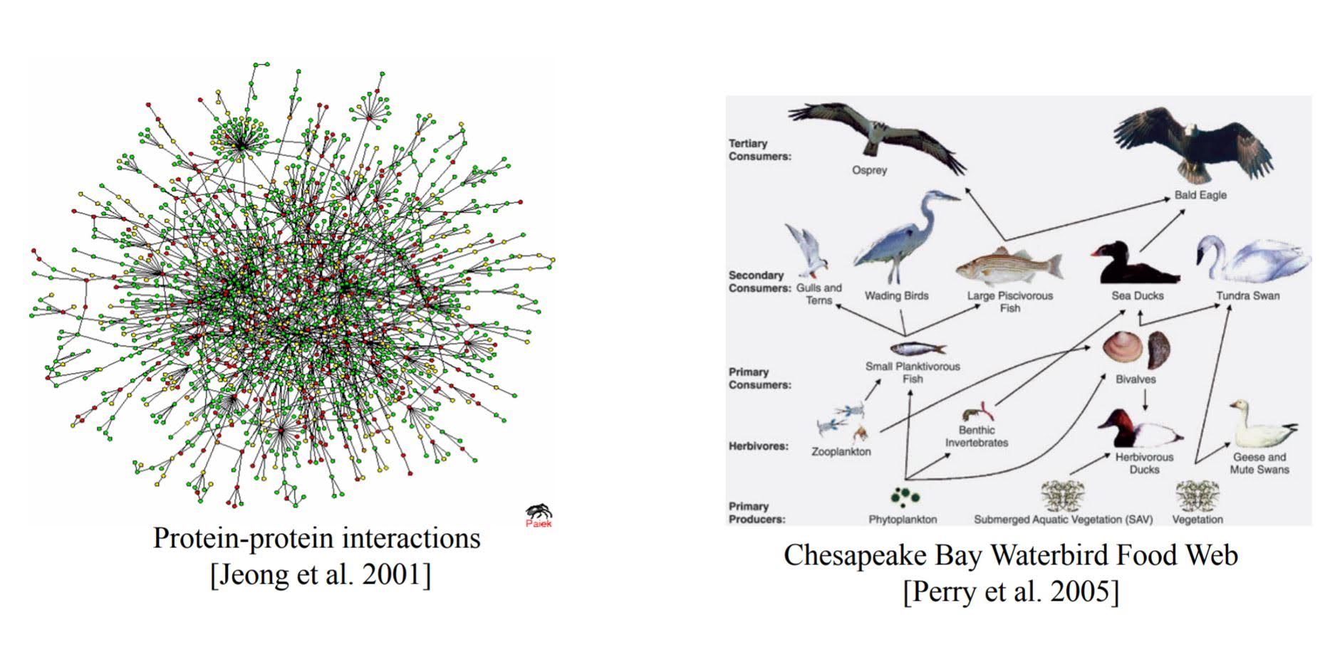
• Biological Networks

Applications of networks

• Is a rumor likely to spread in this network?
• Who are the most influential people in this organization?
• Is this club likely to split into two groups? If so, which nodes will go to which group?
• Which airports are at highest risk for virus spreading?
• Are some parts of the world more difficult to reach?

Basic Concepts

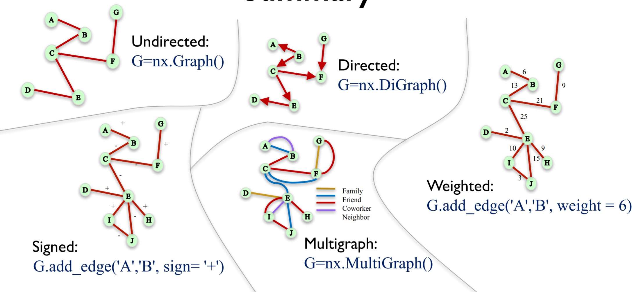
• Node and Edge
• Undirected network: Nodes have symmetric relationships
  Directed network: Nodes have assymmetric relationships
• Weighted network: A network where edges are assigned a weight
• Signed network: A network where edges are assigned positive or negative sign
• Edges can carry many other labels or attributes. Attribute can be weight, sign, relation,…
• Multigraph: a network where multiple edges can connect the same nodes

We will use NetworkX to handle graphs in python.

import networkx as nx
import numpy as np
import pandas as pd
import matplotlib.pyplot as plt
%matplotlib inline

Edge Attributes in NetworkX

Undirected network

G=nx.Graph()
G.add_edge('A','B', weight= 6, relation = 'family')
G.add_edge('B','C', weight= 13, relation = 'friend')
G.edges()

EdgeView([('A', 'B'), ('B', 'C')])

G.edges(data=True)

EdgeDataView([('A', 'B', {'weight': 6, 'relation': 'family'}), ('B', 'C', {'weight': 13, 'relation': 'friend'})])

G.edges(data='weight')

EdgeDataView([('A', 'B', 6), ('B', 'C', 13)])

G['A']

AtlasView({'B': {'weight': 6, 'relation': 'family'}})

G['A']['B']

{'weight': 6, 'relation': 'family'}

G['B']['A']

{'weight': 6, 'relation': 'family'}

Directed network

G=nx.DiGraph()
G.add_edge('A','B', weight= 6, relation = 'family')
G.add_edge('C', 'B', weight= 13, relation = 'friend')

G['C']['B']
# G['B']['C'] will yield KeyError

{'weight': 13, 'relation': 'friend'}

MultiGraph

G=nx.MultiGraph()
G.add_edge('A','B', weight= 6, relation = 'family')
G.add_edge('A','B', weight= 18, relation = 'friend')
G.add_edge('C','B', weight= 13, relation = 'friend')

0

G['A']['B']

AtlasView({0: {'weight': 6, 'relation': 'family'}, 1: {'weight': 18, 'relation': 'friend'}})

Directed MultiGraph

G=nx.MultiDiGraph()
G.add_edge('A','B', weight= 6, relation = 'family')
G.add_edge('A','B', weight= 18, relation = 'friend')
G.add_edge('C','B', weight= 13, relation = 'friend')

0

G['A']['B'][0]['weight']

6

Node Attributes in NetworkX

G=nx.Graph()
G.add_edge('A','B', weight= 6, relation = 'family')
G.add_edge('B','C', weight= 13, relation = 'friend')
# Add node attributes
G.add_node('A', role = 'trader')
G.add_node('B', role = 'trader')
G.add_node('C', role = 'manager')

G.nodes()

NodeView(('A', 'B', 'C'))

G.nodes(data=True)

NodeDataView({'A': {'role': 'trader'}, 'B': {'role': 'trader'}, 'C': {'role': 'manager'}})

G.node['A']

{'role': 'trader'}

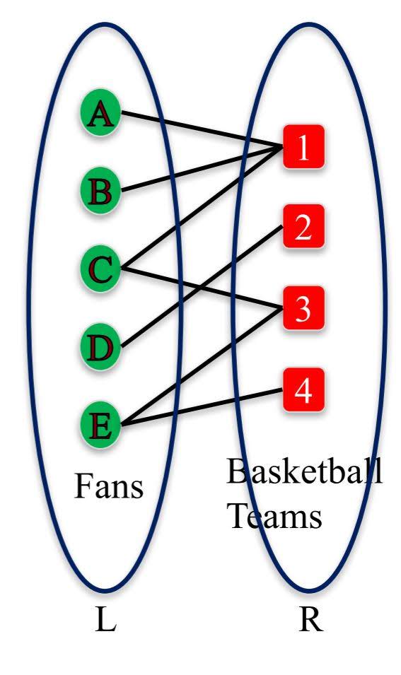
Bipartite Graphs

Bipartite Graph is a graph whose nodes can be split into two sets L and R, and every edge connects an node in L with a node in R.

from networkx.algorithms import bipartite
B = nx.Graph() #No separate class for bipartite graphs
B.add_nodes_from(['A', 'B', 'C', 'D', 'E'], bipartite=0) #label one set of nodes 0
B.add_nodes_from([1,2,3,4], bipartite=1) #label other set of nodes 1
B.add_edges_from([('A',1), ('A', 2), ('B',1), ('C',1), ('C',3), ('D',2), ('E',3), ('E', 4)])

Check if a graph is bipartite

bipartite.is_bipartite(B)

True

Check if a set of nodes is a bipartition of a graph

X = set([1,2,3,4])
bipartite.is_bipartite_node_set(B, X)

True

Get each set of nodes of a bipartite graph

bipartite.sets(B)

({'A', 'B', 'C', 'D', 'E'}, {1, 2, 3, 4})

Projected Graphs

L-Bipartite graph projection: Network of nodes in group L, where a pair of nodes is connected if they have a common neighbor in R in the bipartite graph.
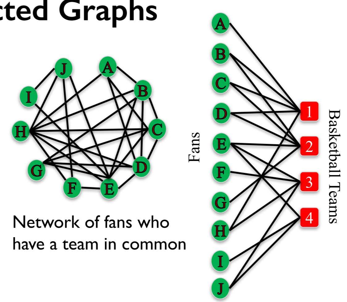
Similar definition for R-Bipartite graph projection

B = nx.Graph()
B.add_edges_from([('A',1), ('B',1),('C',1),('D',1),('H',1), ('B', 2), ('C', 2), ('D',2),('E', 2), ('G', 2), ('E', 3), ('F', 3), ('H', 3), ('J', 3), ('E', 4), ('I', 4), ('J', 4) ])
X = set(['A','B','C','D', 'E', 'F','G', 'H', 'I','J'])
P = bipartite.projected_graph(B, X)
nx.draw_networkx(P)

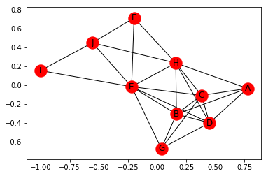
L-Bipartite weighted graph projection: An L-Bipartite graph projection with weights on the edges that are proportional to the number of common neighbors between the nodes.

P = bipartite.weighted_projected_graph(B, X)
P.edges(data = True)

EdgeDataView([('E', 'I', {'weight': 1}), ('E', 'B', {'weight': 1}), ('E', 'D', {'weight': 1}), ('E', 'J', {'weight': 2}), ('E', 'H', {'weight': 1}), ('E', 'C', {'weight': 1}), ('E', 'F', {'weight': 1}), ('E', 'G', {'weight': 1}), ('I', 'J', {'weight': 1}), ('B', 'D', {'weight': 2}), ('B', 'H', {'weight': 1}), ('B', 'A', {'weight': 1}), ('B', 'C', {'weight': 2}), ('B', 'G', {'weight': 1}), ('D', 'H', {'weight': 1}), ('D', 'A', {'weight': 1}), ('D', 'C', {'weight': 2}), ('D', 'G', {'weight': 1}), ('J', 'F', {'weight': 1}), ('J', 'H', {'weight': 1}), ('H', 'A', {'weight': 1}), ('H', 'C', {'weight': 1}), ('H', 'F', {'weight': 1}), ('A', 'C', {'weight': 1}), ('C', 'G', {'weight': 1})])

Various Ways to Load Graphs in NetworkX

1. add_edges_from

# Instantiate the graph
G1 = nx.Graph()
# add node/edge pairs
G1.add_edges_from([(0, 1),
                   (0, 2),
                   (0, 3),
                   (0, 5),
                   (1, 3),
                   (1, 6),
                   (3, 4),
                   (4, 5),
                   (4, 7),
                   (5, 8),
                   (8, 9)])

G1.edges()

EdgeView([(0, 1), (0, 2), (0, 3), (0, 5), (1, 3), (1, 6), (3, 4), (5, 4), (5, 8), (4, 7), (8, 9)])

2. Adjacency List

G_adjlist.txt is the adjaceny list representation of G1.

It can be read as follows:

• 0 1 2 3 5 $\rightarrow$ node 0 is adjacent to nodes 1, 2, 3, 5
• 1 3 6 $\rightarrow$ node 1 is (also) adjacent to nodes 3, 6
• 2 $\rightarrow$ node 2 is (also) adjacent to no new nodes
• 3 4 $\rightarrow$ node 3 is (also) adjacent to node 4

pd.read_csv('G_adjlist.txt', header = None)

	0
0	0 1 2 3 5
1	1 3 6
2	2
3	3 4
4	4 5 7
5	5 8
6	6
7	7
8	8 9
9	9

G2 = nx.read_adjlist('G_adjlist.txt', nodetype=int, create_using = nx.Graph())
G2.edges()

EdgeView([(0, 1), (0, 2), (0, 3), (0, 5), (1, 3), (1, 6), (3, 4), (5, 4), (5, 8), (4, 7), (8, 9)])

We can use argument create_using to specify which NetworkX graph to use when creating graph.

3. Adjacency Matrix

The elements in an adjacency matrix indicate whether pairs of vertices are adjacent or not in the graph. Each node has a corresponding row and column. For example, row 0, column 1 corresponds to the edge between node 0 and node 1.

Reading across row 0, there is a ‘1’ in columns 1, 2, 3, and 5, which indicates that node 0 is adjacent to nodes 1, 2, 3, and 5

G_mat = np.array([[0, 1, 1, 1, 0, 1, 0, 0, 0, 0],
                  [1, 0, 0, 1, 0, 0, 1, 0, 0, 0],
                  [1, 0, 0, 0, 0, 0, 0, 0, 0, 0],
                  [1, 1, 0, 0, 1, 0, 0, 0, 0, 0],
                  [0, 0, 0, 1, 0, 1, 0, 1, 0, 0],
                  [1, 0, 0, 0, 1, 0, 0, 0, 1, 0],
                  [0, 1, 0, 0, 0, 0, 0, 0, 0, 0],
                  [0, 0, 0, 0, 1, 0, 0, 0, 0, 0],
                  [0, 0, 0, 0, 0, 1, 0, 0, 0, 1],
                  [0, 0, 0, 0, 0, 0, 0, 0, 1, 0]])

G3 = nx.Graph(G_mat)
G3.edges()

EdgeView([(0, 1), (0, 2), (0, 3), (0, 5), (1, 3), (1, 6), (3, 4), (4, 5), (4, 7), (5, 8), (8, 9)])

4. Edgelist

The edge list format represents edge pairings in the first two columns. Additional edge attributes can be added in subsequent columns. Looking at G_edgelist.txt this is the same as the original graph G1, but now each edge has a weight.

For example, from the first row, we can see the edge between nodes 0 and 1, has a weight of 4.

pd.read_csv('G_edgelist.txt', header = None)

	0
0	0 1 4
1	0 2 3
2	0 3 2
3	0 5 6
4	1 3 2
5	1 6 5
6	3 4 3
7	4 5 1
8	4 7 2
9	5 8 6
10	8 9 1

G4 = nx.read_edgelist('G_edgelist.txt', data=[('Weight', int)])

G4.edges(data=True)

EdgeDataView([('0', '1', {'Weight': 4}), ('0', '2', {'Weight': 3}), ('0', '3', {'Weight': 2}), ('0', '5', {'Weight': 6}), ('1', '3', {'Weight': 2}), ('1', '6', {'Weight': 5}), ('3', '4', {'Weight': 3}), ('5', '4', {'Weight': 1}), ('5', '8', {'Weight': 6}), ('4', '7', {'Weight': 2}), ('8', '9', {'Weight': 1})])

5. Pandas DataFrame

Graphs can also be created from pandas dataframes if they are in edge list format.

G_df = pd.read_csv('G_edgelist.txt', delim_whitespace=True,
                   header=None, names=['n1', 'n2', 'weight'])
G_df

	n1	n2	weight
0	0	1	4
1	0	2	3
2	0	3	2
3	0	5	6
4	1	3	2
5	1	6	5
6	3	4	3
7	4	5	1
8	4	7	2
9	5	8	6
10	8	9	1

G5 = nx.from_pandas_edgelist(G_df, 'n1', 'n2', edge_attr='weight')
G5.edges(data=True)

EdgeDataView([(0, 1, {'weight': 4}), (0, 2, {'weight': 3}), (0, 3, {'weight': 2}), (0, 5, {'weight': 6}), (1, 3, {'weight': 2}), (1, 6, {'weight': 5}), (3, 4, {'weight': 3}), (5, 4, {'weight': 1}), (5, 8, {'weight': 6}), (4, 7, {'weight': 2}), (8, 9, {'weight': 1})])

Excercise - Employee Relationships and their Movie Choices

Eight employees at a small company were asked to choose 3 movies that they would most enjoy watching for the upcoming company movie night. These choices are stored in the file Employee_Movie_Choices.txt.

A second file, Employee_Relationships.txt, has data on the relationships between different coworkers.

The relationship score has value of -100 (Enemies) to +100 (Best Friends). A value of zero means the two employees haven’t interacted or are indifferent.

Both files are tab delimited.

# This is the set of employees
employees = set(['Pablo',
                 'Lee',
                 'Georgia',
                 'Vincent',
                 'Andy',
                 'Frida',
                 'Joan',
                 'Claude'])

# This is the set of movies
movies = set(['The Shawshank Redemption',
              'Forrest Gump',
              'The Matrix',
              'Anaconda',
              'The Social Network',
              'The Godfather',
              'Monty Python and the Holy Grail',
              'Snakes on a Plane',
              'Kung Fu Panda',
              'The Dark Knight',
              'Mean Girls'])

Using NetworkX, load in the bipartite graph from Employee_Movie_Choices.txt and return that graph.

employee_movie_choices = pd.read_csv('Employee_Movie_Choices.txt', sep="\t")
employee_movie_choices.head()

	#Employee	Movie
0	Andy	Anaconda
1	Andy	Mean Girls
2	Andy	The Matrix
3	Claude	Anaconda
4	Claude	Monty Python and the Holy Grail

B = nx.from_pandas_edgelist(employee_movie_choices, '#Employee', 'Movie')
B.edges()

EdgeView([('Andy', 'Anaconda'), ('Andy', 'Mean Girls'), ('Andy', 'The Matrix'), ('Anaconda', 'Claude'), ('Anaconda', 'Georgia'), ('Mean Girls', 'Joan'), ('Mean Girls', 'Lee'), ('The Matrix', 'Frida'), ('The Matrix', 'Pablo'), ('Claude', 'Monty Python and the Holy Grail'), ('Claude', 'Snakes on a Plane'), ('Monty Python and the Holy Grail', 'Georgia'), ('Snakes on a Plane', 'Georgia'), ('Frida', 'The Shawshank Redemption'), ('Frida', 'The Social Network'), ('The Shawshank Redemption', 'Pablo'), ('The Shawshank Redemption', 'Vincent'), ('The Social Network', 'Vincent'), ('Joan', 'Forrest Gump'), ('Joan', 'Kung Fu Panda'), ('Forrest Gump', 'Lee'), ('Kung Fu Panda', 'Lee'), ('Pablo', 'The Dark Knight'), ('Vincent', 'The Godfather')])

Add nodes attributes named 'type' where movies have the value 'movie' and employees have the value 'employee'.

for employee in employees:
    nx.set_node_attributes(B, {employee: {'type':'employee'}})
for movie in movies:
    nx.set_node_attributes(B, {movie: {'type':'movie'}})

nx.get_node_attributes(B, 'type')

{'Andy': 'employee',
 'Anaconda': 'movie',
 'Mean Girls': 'movie',
 'The Matrix': 'movie',
 'Claude': 'employee',
 'Monty Python and the Holy Grail': 'movie',
 'Snakes on a Plane': 'movie',
 'Frida': 'employee',
 'The Shawshank Redemption': 'movie',
 'The Social Network': 'movie',
 'Georgia': 'employee',
 'Joan': 'employee',
 'Forrest Gump': 'movie',
 'Kung Fu Panda': 'movie',
 'Lee': 'employee',
 'Pablo': 'employee',
 'The Dark Knight': 'movie',
 'Vincent': 'employee',
 'The Godfather': 'movie'}

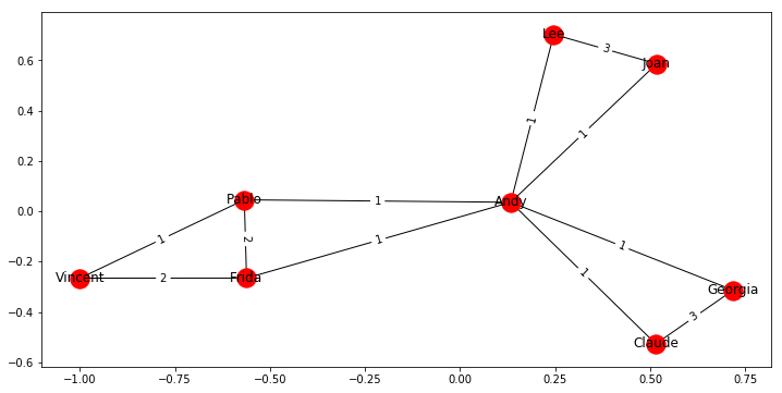
Find a weighted projection of the graph B which tells us how many movies different pairs of employees have in common.

G = bipartite.weighted_projected_graph(B, employees)

#draw weighted projected graph
plt.figure(figsize=(12, 6))
pos = nx.spring_layout(G)
labels = nx.get_edge_attributes(G,'weight')
nx.draw_networkx(G, pos)
nx.draw_networkx_edge_labels(G, pos, edge_labels=labels)

{('Andy', 'Joan'): Text(0.325218,0.311241,'1'),
 ('Andy', 'Frida'): Text(-0.214194,-0.114758,'1'),
 ('Andy', 'Lee'): Text(0.189784,0.369681,'1'),
 ('Andy', 'Pablo'): Text(-0.217167,0.0408515,'1'),
 ('Andy', 'Claude'): Text(0.323979,-0.245456,'1'),
 ('Andy', 'Georgia'): Text(0.425663,-0.138723,'1'),
 ('Joan', 'Lee'): Text(0.381689,0.644936,'3'),
 ('Frida', 'Vincent'): Text(-0.780851,-0.265623,'2'),
 ('Frida', 'Pablo'): Text(-0.564675,-0.109892,'2'),
 ('Vincent', 'Pablo'): Text(-0.783824,-0.110014,'1'),
 ('Claude', 'Georgia'): Text(0.616329,-0.420165,'3')}

Suppose you’d like to find out if people that have a high relationship score also like the same types of movies.
Find the Pearson correlation ( using DataFrame.corr() ) between employee relationship scores and the number of movies they have in common. If two employees have no movies in common it should be treated as a 0, not a missing value, and should be included in the correlation calculation.

employee_relationships = pd.read_csv('Employee_Relationships.txt', sep="\t", header=None)
employee_relationships.tail()

	0	1	2
23	Joan	Pablo	0
24	Joan	Vincent	10
25	Lee	Pablo	0
26	Lee	Vincent	0
27	Pablo	Vincent	-20

employee_relationships = employee_relationships.set_index([0, 1])
employee_relationships.tail()

		2
0	1
Joan	Pablo	0
	Vincent	10
Lee	Pablo	0
	Vincent	0
Pablo	Vincent	-20

weights = nx.get_edge_attributes(G,'weight')
weights

{('Andy', 'Joan'): 1,
 ('Andy', 'Frida'): 1,
 ('Andy', 'Lee'): 1,
 ('Andy', 'Pablo'): 1,
 ('Andy', 'Claude'): 1,
 ('Andy', 'Georgia'): 1,
 ('Joan', 'Lee'): 3,
 ('Frida', 'Vincent'): 2,
 ('Frida', 'Pablo'): 2,
 ('Vincent', 'Pablo'): 1,
 ('Claude', 'Georgia'): 3}

for index, weight in weights.items():
    if index in list(employee_relationships.index):
        employee_relationships.loc[index, 'weight'] = weight
    else:
        employee_relationships.loc[(index[1], index[0]), 'weight'] = weight
employee_relationships.tail()

		2	weight
0	1
Joan	Pablo	0	NaN
	Vincent	10	NaN
Lee	Pablo	0	NaN
	Vincent	0	NaN
Pablo	Vincent	-20	1.0

employee_relationships = employee_relationships.fillna(0)
corr = employee_relationships.corr()
corr

	2	weight
2	1.000000	0.788396
weight	0.788396	1.000000

corr.iloc[0,1]

0.7883962221733476