Influence Measures and Network Centrality

Original Source: https://www.coursera.org/specializations/data-science-python

Network Centrality

Centrality measures identify the most important nodes in a network.

Examples in real world

• Influential nodes in a social network.
• Nodes that disseminate information to many nodes or prevent epidemics.
• Hubs in a transportation network.
• Important pages on the Web.
• Nodes that prevent the network from breaking up.

There are different ways to measure centrality of a node.

• Degree centrality
• Closeness centrality
• Betweenness centrality
• Page Rank
• HITS Algorithm

1. Degree Centrality

Assumption: important nodes have many connections

For undirected networks

$ C_{deg}(v) = \frac{d_v}{|N|-1} $, where N is the set of nodes in the network and $d_v$ is the degree of node v

import networkx as nx
import matplotlib.pyplot as plt
%matplotlib inline

G = nx.karate_club_graph()

def draw_network(G):    
    plt.figure(figsize=(12,7))
    nx.draw_networkx(G, alpha=0.6, node_size = 1000, font_size=16, edge_color='.4')
    plt.axis('off')
    plt.tight_layout();

draw_network(G)

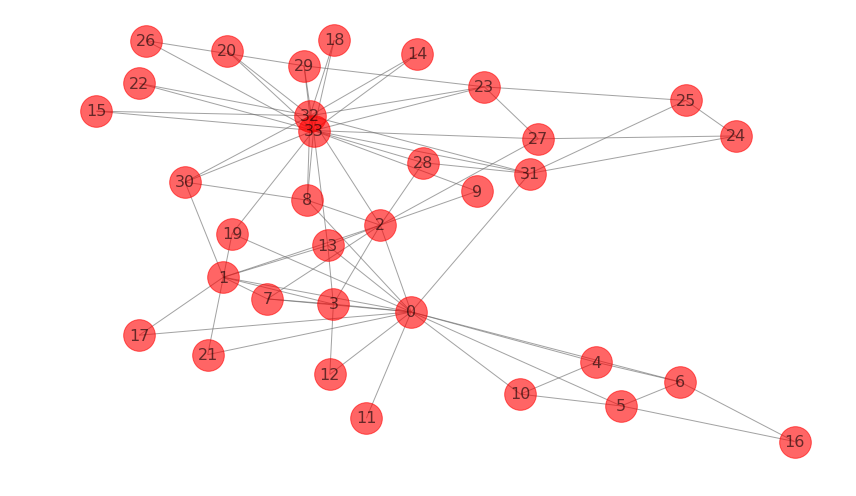
centrality = nx.degree_centrality(G)
# top 5 pairs of (node, degree_centrality)
sorted(centrality.items(), key=lambda x: x[1], reverse=True)[:5]

[(33, 0.5151515151515151),
 (0, 0.48484848484848486),
 (32, 0.36363636363636365),
 (2, 0.30303030303030304),
 (1, 0.2727272727272727)]

For directed networks

1. in-degree centrality

$ C_{deg}^{in}(v) = \frac{d_v}{|N|-1} $, where N is the set of nodes in the network and $d_v$ is the in-degree of node v

G_di = nx.DiGraph()
G_di.add_edges_from([('A', 'B'), ('C', 'A'), ('A', 'E'), ('G', 'J'), ('G', 'A'), ('D', 'B'), ('B', 'E'), ('B' 'C'), ('C', 'D'), ('E', 'C'), ('E', 'D'), ('F', 'G'), ('I', 'F'), ('J', 'F'), ('I', 'J'), ('I', 'H'), ('H', 'I'), ('I', 'G'), ('H', 'G'), ('O', 'J'), ('J', 'O'), ('A', 'N'), ('L', 'M'), ('K', 'M'), ('K', 'L'), ('N', 'L'), ('O', 'L'), ('O', 'K'), ('N', 'O')])
draw_network(G_di)

centrality = nx.in_degree_centrality(G_di)
# top 5 pairs of (node, centrality)
sorted(centrality.items(), key=lambda x: x[1], reverse=True)[:5]

[('G', 0.21428571428571427),
 ('J', 0.21428571428571427),
 ('L', 0.21428571428571427),
 ('A', 0.14285714285714285),
 ('B', 0.14285714285714285)]

2. out-degree centrality

$ C_{deg}^{out}(v) = \frac{d_v}{|N|-1} $, where N is the set of nodes in the network and $d_v$ is the out-degree of node v

centrality = nx.out_degree_centrality(G_di)
# top 5 pairs of (node, centrality)
sorted(centrality.items(), key=lambda x: x[1], reverse=True)[:5]

[('I', 0.2857142857142857),
 ('A', 0.21428571428571427),
 ('O', 0.21428571428571427),
 ('B', 0.14285714285714285),
 ('C', 0.14285714285714285)]

2. Closeness Centrality

Assumption: important nodes are close to other nodes

$ C_{close}(v) = \frac{|R(v)|}{|N-1|} \frac{|R(v)|}{\sum_{u,v\in R(v)} d(v,u)} $, where $ N $ is the set of nodes in the network, $ R(v) $ is the set of nodes v can reach, and $ d(v,u) $ is the length of shortest path from v to u.

We multiply $ \frac{|R(v)|}{|N-1|} $ to penalize centrality of a node that has small number of nodes it can reach(that has small R(v)).
For example in the above graph G_di, if we do not multiply normalization term, centrality of node ‘L’ is 1, which is too high for a node that can only reach one other node.

centrality = nx.closeness_centrality(G)
# top 5 pairs of (node, centrality)
sorted(centrality.items(), key=lambda x: x[1], reverse=True)[:5]

[(0, 0.5689655172413793),
 (2, 0.559322033898305),
 (33, 0.55),
 (31, 0.5409836065573771),
 (8, 0.515625)]

3. Betweenness Centrality

Assumption: important nodes connect other nodes

$ C_{btw}(v) = \sum_{s,t\in R} \frac{\sigma_{s,t}(v)}{\sigma_{s,t}} $, where $ R $ is the set of two nodes which are connected, $ \sigma_{s,t} $ is the number of shortest paths between nodes s and t, and $ \sigma_{s,t}(v) $ is the number of shortest paths between nodes s and t that pass through node v.

There are 3 options when computing betweenness centrality.

1. endpoints
   When computing betweenness centrality of a node $ v $, we can either include or exclude paths that have $ v $ in endpoints $ s $ or $ t $.
2. normalization
   betwenness centrality values will be larger in graphs with many nodes. To control this, we divide centrality values by the number of pairs of nodes in the graph (excluding v).
   Dividing term is as follows.
   $ \frac{1}{2}(|N|-1)(|N|-2) $ in undirected graphs
   $ (|N|-1)(|N|-2) $ in directed graphs
3. k (approximation)
   Computing betweenness centrality of all nodes can be very computationally expensive. Depending on the algorithm, this computation can take up to $ O({|N|}^3) $ time.
   So rather can computing betweenness centrality based on all pairs of nodes s, t, we can approximate it based on a sample of nodes.

centrality = nx.betweenness_centrality(G, normalized=True, endpoints=False, k=10)
# top 5 pairs of (node, centrality)
sorted(centrality.items(), key=lambda x: x[1], reverse=True)[:5]

[(0, 0.44680450336700334),
 (33, 0.2966874098124098),
 (31, 0.20575907888407888),
 (32, 0.17188071188071188),
 (5, 0.06439393939393939)]

Betweenness Centrality between subsets

We can calculate betweenness centrality between subsets of a network. When counting shortest paths, we only consider paths that start from one of the nodes in subset A and end at one of the nodes in subset B.

centrality = nx.betweenness_centrality_subset(G, [32, 33, 21, 30, 16, 27, 15, 23, 10], [1, 4, 13, 11, 6, 12, 17, 7])
# top 5 pairs of (node, centrality)
sorted(centrality.items(), key=lambda x: x[1], reverse=True)[:5]

[(0, 21.609126984126988),
 (2, 8.27845238095238),
 (33, 5.183888888888888),
 (1, 4.2630952380952385),
 (8, 3.1306349206349204)]

Betweenness Centrality of Edges

centrality = nx.edge_betweenness_centrality(G)
# top 5 pairs of (node, centrality)
sorted(centrality.items(), key=lambda x: x[1], reverse=True)[:5]

[((0, 31), 0.1272599949070537),
 ((0, 6), 0.07813428401663695),
 ((0, 5), 0.07813428401663694),
 ((0, 2), 0.0777876807288572),
 ((0, 8), 0.07423959482783014)]

4. PageRank

PageRank algorithm is developed by Google founders to measure the importance of webpages from the hyperlink network structure.
PageRank assigns a score of importance to each node. Important nodes are those with many in-links from important pages.
PageRank can be used for any type of network, but it is mainly useful for directed networks.

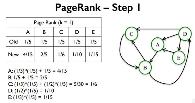
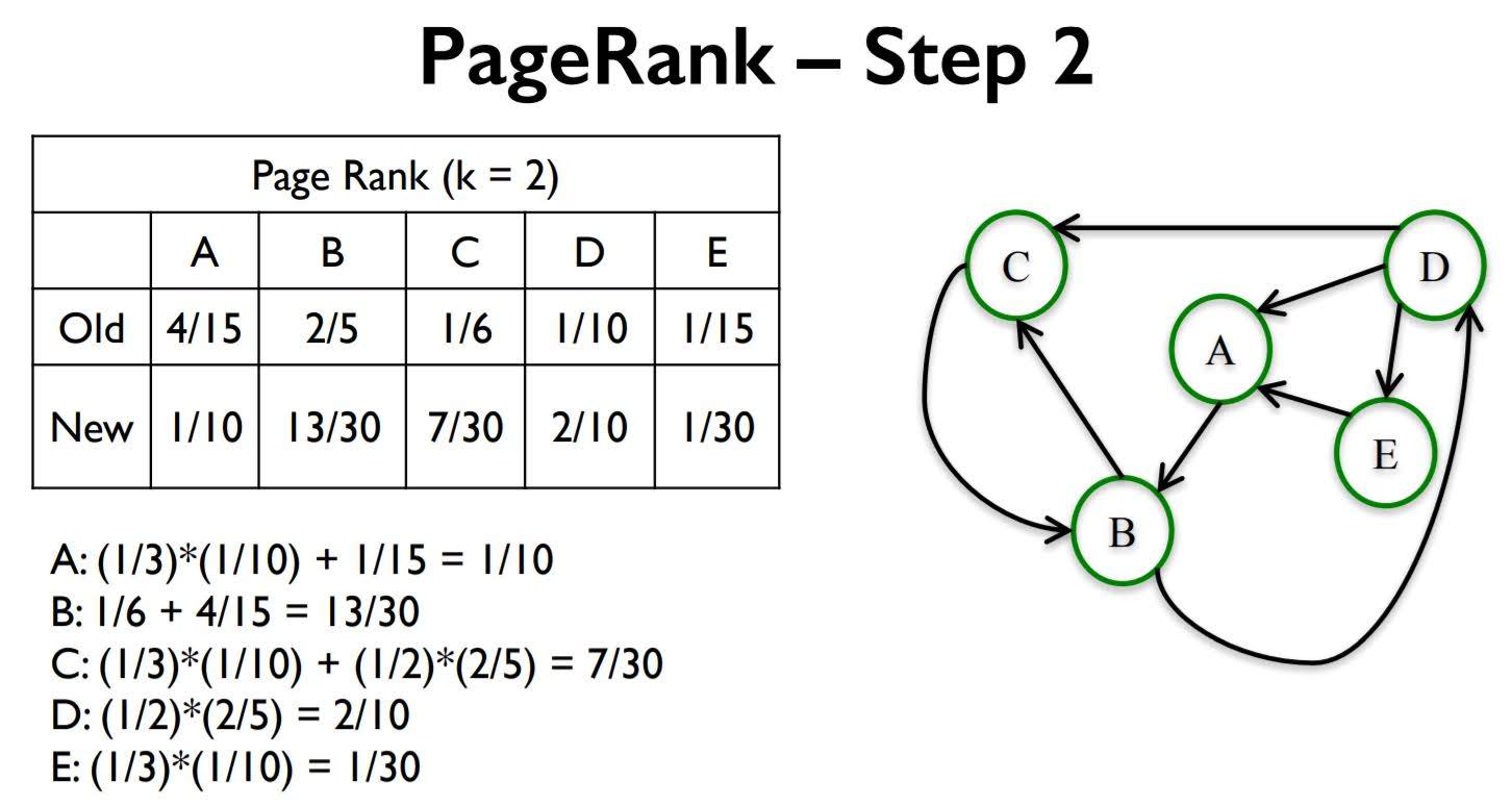
Basic PageRank

In basic PageRank, we repeat the following rule infinitly to get importance of a certain page. For most networks, PageRank values converge as k(number of repetition) gets larger.

Basic PageRank Update Rule
Each node gives an equal share of its current PageRank to all the nodes it links to. The new PageRank of each node is the sum of all the PageRank it received from other nodes.

Example

Interpreting PageRank as Random walk of k steps

Random walk: Start on a random node. Then choose an outgoing edge at random and follow it to the next node. Repeat k times.
The probabilty of node ‘a’ being current node at step k equals to PageRank of node ‘a’ at step k.

Scaled Page Rank

PageRank Problem

In the above graph, for a large enough k: F and G each have PageRank of 1/2 and all the other nodes have PageRank 0.

To fix this problem, we introduce a ‘damping parameter’ $ \alpha $

Scaled PageRank Random walk
Start on a random node. Then:

• With probability $ \alpha $: choose an outgoing edge at random and follow it to the next node.
• With probability 1 − $ \alpha $: choose a node at random and go to it.

The Scaled PageRank of k steps and damping factor $ \alpha $ of a node n is the probability that a random walk with damping facto r$ \alpha $ lands on a n after k steps.

In practice, we use a parameter of $ \alpha $ between 0.8 and 0.9.

After setting $ \alpha $ to 0.8, nodes other than F or G in the above graph get PageRank bigger than 0.

# Note that G_di is not the above graph.
centrality = nx.pagerank(G_di, alpha=0.8)
# top 5 pairs of (node, centrality)
sorted(centrality.items(), key=lambda x: x[1], reverse=True)[:5]

[('B', 0.1136679799498734),
 ('C', 0.09765860364475079),
 ('D', 0.09125558981288656),
 ('E', 0.08613006508366944),
 ('A', 0.08596118308469886)]

5. Hubs and Authorities (HITS Algorithm)

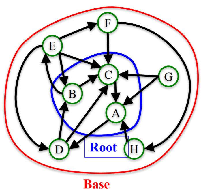
Before assigning rank to pages, we need to pick pages that are relevant to the query. We call relevant pages and their connections ‘Base’. This is how we find base.
Given a query to a search engine:

• Root: set of highly relevant web pages (e.g. pages that contain the query string) – potential authorities.
• Find all pages that link to a page in root – potential hubs.
• Base: root nodes and any node that links to a node in root.
• Consider all edges connecting nodes in the base set.

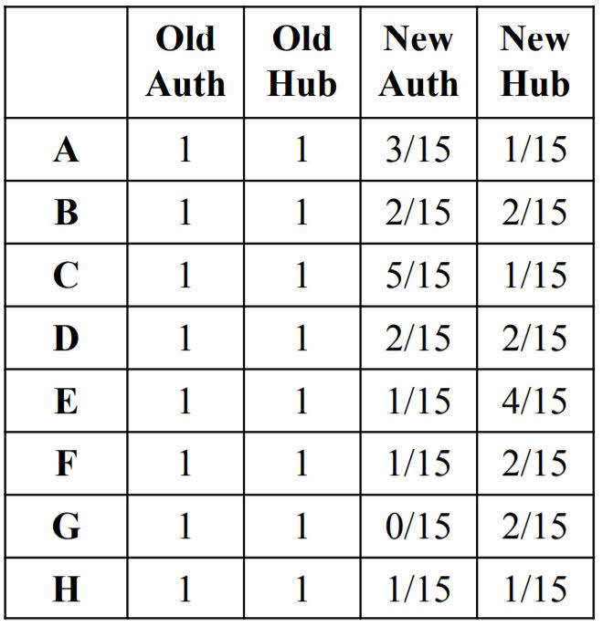
After finding base, Computing k iterations of the HITS algorithm to assign an ‘authority score’ and ‘hub score’ to each node.

1. Assign each node an authority and hub score of 1.
2. Apply the Authority Update Rule: each node’s authority score is the sum of hub scores of each node that points to it.
3. Apply the Hub Update Rule: each node’s hub score is the sum of authority scores of each node that it points to.
4. Nomalize Authority and Hub scores: $ auth(J) := \frac{auth(j)}{sum_{i\in N} auth(i)} $
5. Repeat k times.

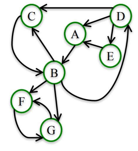
One step of HITS Algorithm

For most networks, as k gets larger, authority and hub scores converge to a unique value.

# note that G_di is not the above graph
# nx.hits returns (hub scores dictionary, auth scores dictionary)
centrality = nx.hits(G_di)

# top 5 pairs of (node, centrality) by hub measurement
hub_scores = centrality[0]
print(sorted(hub_scores.items(), key=lambda x: x[1], reverse=True)[:5])

# top 5 pairs of (node, centrality) by hub measurement
auth_scores = centrality[1]
print(sorted(auth_scores.items(), key=lambda x: x[1], reverse=True)[:5])

[('I', 0.2633434794139307), ('O', 0.17579324129888213), ('G', 0.11714778282617944), ('J', 0.08601213301577858), ('H', 0.08277050829140217)]
[('J', 0.2122699074081906), ('G', 0.15840540582653959), ('F', 0.13330891475417173), ('L', 0.12416151353124302), ('H', 0.10048796182090457)]

Centrality Measures Comparison

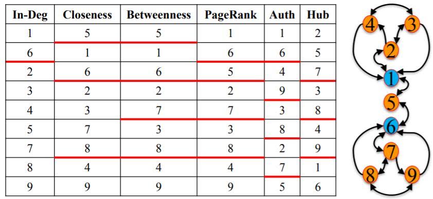
The best centrality measure depends on the context of the network one is analyzing.
When identifying central nodes, it is usually best to use multiple centrality measures instead of relying on a single one.