
Network Evolution (Preferential Attachment Model, Small World Model, Link Prediction)
Original Source: https://www.coursera.org/specializations/data-science-python
Degree Distributions
The degree of a node in an undirected graph is the number of neighbors it has.
The degree distribution of a graph is the probability distribution of the degrees over the entire network.
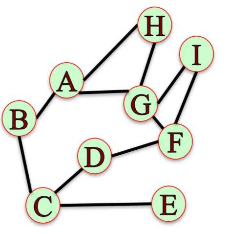
The degree distribution, $P(k)$, of the above network has the following values:
$P(1)=\frac{1}{9}, P(2)=\frac{4}{9}, P(3)=\frac{1}{3}, P(4)=\frac{1}{9}$
Directed Graph
Basically same as degree in undirected graph. Only difference is that there are in-degree (distribution) and out-degree (distribution).
import networkx as nx
import matplotlib.pyplot as plt
import seaborn as sns
sns.set()
%matplotlib inline
G=nx.Graph()
G.add_edges_from([('A','B'), ('A','G'), ('A','H'), ('B','C'), ('C','D'), ('C','E'), ('D','F'), ('F','G'), ('G','H'), ('G','I')])
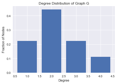
degrees = dict(G.degree()) # for directed graphs, G.in-degree() or G.out-degree()
degree_values = sorted(set(degrees.values()))
histogram = [list(degrees.values()).count(i)/float(nx.number_of_nodes(G)) for i in degree_values]
plt.figure()
plt.bar(degree_values,histogram)
plt.title('Degree Distribution of Graph G')
plt.xlabel('Degree')
plt.ylabel('Fraction of Nodes')
plt.show()
Degree Distributions in Real Networks
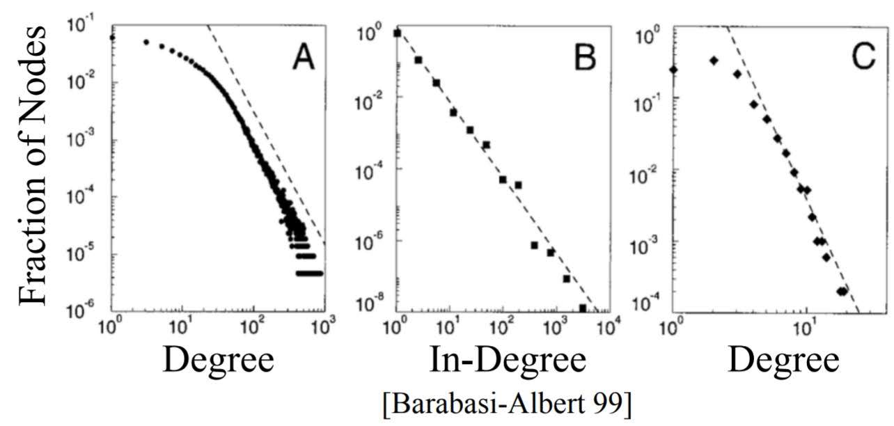
B – The Web: network of 325,000 documents on the WWW connected by URLs.
C – US Power Grid: network of 4,941 generators connected by transmission lines.
Degree distributions in real world tend to look like a straight line when on a log-log scale(both x and y axis are on log scale) as shown above. They tend to follow ‘Power Law’.
Power law: $P(k)=Ck^{-\alpha}$, where $\alpha$ and $C$ are constants.
Networks with power law distribution have many nodes with small degree and a few nodes with very large degree.
Preferential Attachment Model
Preferential Attachment Model explains how networks that follow power law were created.
How does this model creates networks?
- Start with two nodes connected by an edge.
- At each time step, add a new node with an edge connecting it to an existing node.
- Choose the node to connect to at random with probability proportional to each node’s degree.
- The probability of connecting to a node $u$ of degree $k_u$ is $\frac{k_u}{\sum_j k_j}$.
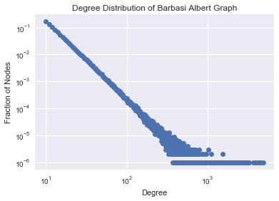
As the number of nodes increases, the degree distribution of the network under the preferential attachment model approaches the power law $P(k)=Ck^{-3}$.
Application in Networkx
Specifically we can use nx.barabasi_albert_graph in networkx to produce such graphs.
barabasi_albert_graph(n, m) returns a network with n nodes. Each new node attaches to m existing nodes according to the Preferential Attachment model.
G = nx.barabasi_albert_graph(1000000,10)

degrees = dict(G.degree())
degree_values = sorted(set(degrees.values()))
histogram = [list(degrees.values()).count(i)/float(nx.number_of_nodes(G)) for i in degree_values]

plt.figure()
plt.plot(degree_values,histogram, 'o')
plt.title('Degree Distribution of Barbasi Albert Graph')
plt.xlabel('Degree')
plt.ylabel('Fraction of Nodes')
plt.xscale('log')
plt.yscale('log')
plt.show()
Small World Networks
‘Small World’ networks has two properties.
- Average length of shortest paths between possible pairs of nodes in a network is small.
- Clustering coefficient is small. (Local clustering coefficient of a node is fraction of pairs of the node’s friends that are friends with each other.)
Proofs of Small World
1. Milgram Small World Experiment (1960)
296 randomly chosen “starters” were asked to forward a letter to a “target” person. Target was a stockbroker in Boston.
Instructions for starter:
- Send letter to target if you know him on a first name basis.
- If you do not know target, send letter (and instructions) to someone you know on a first name basis who is more likely to know the target. Some information about the target, such as city, and occupation, was provided.
Result: Median chain length was 6.
2. Microsoft Instant Messenger (2008)
Nodes: 240 million active users on Microsoft Instant Messenger.
Edges: Users engaged in two-way communication over a one-month period.
Result: Estimated median path length of 7.
3. Facebook Global Network (2012)
Result: Average path length in 2008 was 5.28 and in 2011 it was 4.74.
4. Real World Cases of Low Clustering Coefficient
- Facebook 2011: High average CC (decreases with degree; 0.5 when degree=2, 0.2 when degree=50 …)
- Microsoft Instant Message: Average CC of 0.13.
- IMDB actor network: Average CC 0.78
Does Preferential Attachment Model Reproduces Small World?
Graphs created by Preferential Attachment model have small average shortest path length. But since no mechanism in the Preferential Attachment model favors triangle formation, it had low average clustering.
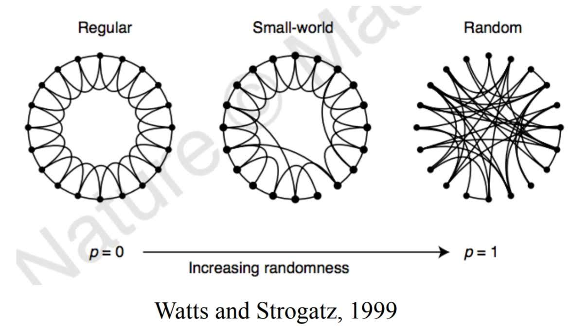
Small World Model
Small World Model was designed to accomplish two properties of Small World Network; high clustering coefficient and small average shortest paths.
How does this model creates networks?
- Start with a ring of $n$ nodes, where each node is connected to its $k$ nearest neighbors.
- Fix a parameter $p\in[0,1]$.
- Consider each edge $(u,v)$. With probability $p$, select a node $w$ at random and rewire the edge $(u,v)$ so it becomes $(u,w)$.
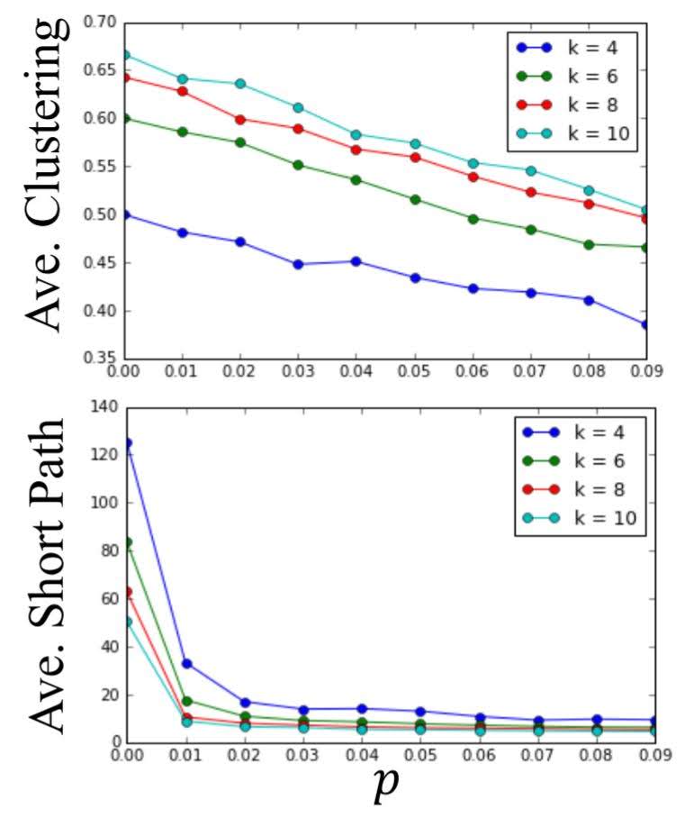
Variable $p$
The resulting network varies with value $p$ as shown below.
As $p$ increases from 0 to 0.01:
- average shortest path decreases rapidly.
- average clustering coefficient deceases slowly.
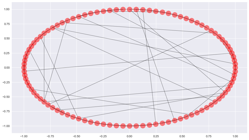
Application in Networkx
We can use nx.watts_strogatz_graph in networkx to produce such graphs.
watts_strogatz_graph(n, k, p) returns a small world network with n nodes, starting with a ring lattice with each node connected to its k nearest neighbors, and rewiring probability p.
G = nx.watts_strogatz_graph(100,5,0.1)
print('average shortest path length: {}'.format(nx.average_shortest_path_length(G)))
print('average clustering coefficient: {}'.format(nx.average_clustering(G)))
plt.figure(figsize=(14, 8))
nx.draw_networkx(G, pos=nx.circular_layout(G), with_labels=False, alpha=0.5)
average shortest path length: 4.893535353535354
average clustering coefficient: 0.36333333333333334
Small world networks can be disconnected, which is sometime undesirable. connected_watts_strogatz_graph(n, k, p, t) runs watts_strogatz_graph(n, k, p) up to t times, until it returns a connected small world network.
newman_watts_strogatz_graph(n, k, p) runs a model similar to the small world model, but rather than rewiring edges, new edges are added with probability p.
Link Prediction
Given a pair of nodes, how can we assess whether they are likely to connect?
Ideas are based on ‘Triadic Closure’, which is the tendency for people who share connections in a social network to become connected.
I’ll introduce 7 measures, 5 of which are commonly applicable and 2 applicable if given specific information.
The graph I will use is shown below.
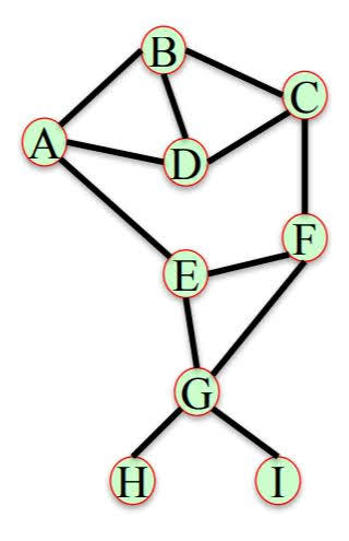
$N(X)$ is the set of neighbors of node $X$.
1. Common Neighbors
$comm neigh(X,Y)=|N(X)\cap N(Y)|$
G = nx.Graph()
G.add_edges_from([('A','B'), ('A','D'), ('A','E'), ('B','C'), ('B','D'), ('C','D'), ('C','F'), ('E','F'), ('E','G'), ('G','F'), ('G','I'), ('G','H')])

# Targets are pairs of nodes that are not connected directly by an edge.
targets = nx.non_edges(G)
common_neigh = [(e[0], e[1], len(list(nx.common_neighbors(G, e[0], e[1])))) for e in targets]
sorted(common_neigh, key=lambda x: x[2], reverse=True)
[('C', 'A', 2),
 ('H', 'I', 1),
 ('H', 'F', 1),
 ('H', 'E', 1),
 ('D', 'F', 1),
 ('D', 'E', 1),
 ('G', 'C', 1),
 ('G', 'A', 1),
 ('C', 'E', 1),
 ('I', 'F', 1),
 ('I', 'E', 1),
 ('B', 'F', 1),
 ('B', 'E', 1),
 ('F', 'A', 1),
 ('H', 'D', 0),
 ('H', 'C', 0),
 ('H', 'B', 0),
 ('H', 'A', 0),
 ('D', 'G', 0),
 ('D', 'I', 0),
 ('G', 'B', 0),
 ('C', 'I', 0),
 ('I', 'B', 0),
 ('I', 'A', 0)]
2. Jaccard Coefficient
$jacc coeff(X,Y)=\frac{|N(X)\cap N(Y)|}{|N(X)\cup N(Y)|}$
jaccard_coefficient = list(nx.jaccard_coefficient(G))
sorted(jaccard_coefficient, key=lambda x: x[2], reverse=True)
[('H', 'I', 1.0),
 ('C', 'A', 0.5),
 ('H', 'F', 0.3333333333333333),
 ('H', 'E', 0.3333333333333333),
 ('I', 'F', 0.3333333333333333),
 ('I', 'E', 0.3333333333333333),
 ('D', 'F', 0.2),
 ('D', 'E', 0.2),
 ('C', 'E', 0.2),
 ('B', 'F', 0.2),
 ('B', 'E', 0.2),
 ('F', 'A', 0.2),
 ('G', 'C', 0.16666666666666666),
 ('G', 'A', 0.16666666666666666),
 ('H', 'D', 0.0),
 ('H', 'C', 0.0),
 ('H', 'B', 0.0),
 ('H', 'A', 0.0),
 ('D', 'G', 0.0),
 ('D', 'I', 0.0),
 ('G', 'B', 0.0),
 ('C', 'I', 0.0),
 ('I', 'B', 0.0),
 ('I', 'A', 0.0)]
3. Resource Allocation
Fraction of a ‘resource’ that a node can send to another through their common neighbors.
$res alloc(X,Y)=\sum_{u\in{N(X)\cap N(Y)}}\frac{1}{|N(u)|}$
resource_allocation_index = list(nx.resource_allocation_index(G))
sorted(resource_allocation_index, key=lambda x: x[2], reverse=True)
[('C', 'A', 0.6666666666666666),
 ('D', 'F', 0.3333333333333333),
 ('D', 'E', 0.3333333333333333),
 ('G', 'C', 0.3333333333333333),
 ('G', 'A', 0.3333333333333333),
 ('C', 'E', 0.3333333333333333),
 ('B', 'F', 0.3333333333333333),
 ('B', 'E', 0.3333333333333333),
 ('F', 'A', 0.3333333333333333),
 ('H', 'I', 0.25),
 ('H', 'F', 0.25),
 ('H', 'E', 0.25),
 ('I', 'F', 0.25),
 ('I', 'E', 0.25),
 ('H', 'D', 0),
 ('H', 'C', 0),
 ('H', 'B', 0),
 ('H', 'A', 0),
 ('D', 'G', 0),
 ('D', 'I', 0),
 ('G', 'B', 0),
 ('C', 'I', 0),
 ('I', 'B', 0),
 ('I', 'A', 0)]
4. Adamic-Adar Index
Similar to resource allocation index, but with log in the denominator.
$adamic adar(X,Y)=\sum_{u\in{N(X)\cap N(Y)}}\frac{1}{\log(|N(u)|)}$
adamic_adar_index = list(nx.adamic_adar_index(G))
sorted(adamic_adar_index, key=lambda x: x[2], reverse=True)
[('C', 'A', 1.8204784532536746),
 ('D', 'F', 0.9102392266268373),
 ('D', 'E', 0.9102392266268373),
 ('G', 'C', 0.9102392266268373),
 ('G', 'A', 0.9102392266268373),
 ('C', 'E', 0.9102392266268373),
 ('B', 'F', 0.9102392266268373),
 ('B', 'E', 0.9102392266268373),
 ('F', 'A', 0.9102392266268373),
 ('H', 'I', 0.7213475204444817),
 ('H', 'F', 0.7213475204444817),
 ('H', 'E', 0.7213475204444817),
 ('I', 'F', 0.7213475204444817),
 ('I', 'E', 0.7213475204444817),
 ('H', 'D', 0),
 ('H', 'C', 0),
 ('H', 'B', 0),
 ('H', 'A', 0),
 ('D', 'G', 0),
 ('D', 'I', 0),
 ('G', 'B', 0),
 ('C', 'I', 0),
 ('I', 'B', 0),
 ('I', 'A', 0)]
5. Pref.Attachment
$pref attach(X,Y)=|N(X)||N(Y)|$
preferential_attachment = list(nx.preferential_attachment(G))
sorted(preferential_attachment, key=lambda x: x[2], reverse=True)
[('D', 'G', 12),
 ('G', 'B', 12),
 ('G', 'C', 12),
 ('G', 'A', 12),
 ('D', 'F', 9),
 ('D', 'E', 9),
 ('C', 'A', 9),
 ('C', 'E', 9),
 ('B', 'F', 9),
 ('B', 'E', 9),
 ('F', 'A', 9),
 ('H', 'D', 3),
 ('H', 'C', 3),
 ('H', 'B', 3),
 ('H', 'F', 3),
 ('H', 'E', 3),
 ('H', 'A', 3),
 ('D', 'I', 3),
 ('C', 'I', 3),
 ('I', 'B', 3),
 ('I', 'F', 3),
 ('I', 'E', 3),
 ('I', 'A', 3),
 ('H', 'I', 1)]
Some measures consider the community structure of the network for link prediction.
Assume the nodes in this network belong to different communities (sets of nodes).
Pairs of nodes who belong to the same community and have many common neighbors in their community are likely to form an edge.
In our graph G, let’s assume that there are two communities, {A,B,C,D} and {E,F,G,H,I}.
6. Community Common Neighbors
$cn soundarajan hopcroft(X,Y)=|N(X)\cap N(Y)|+\sum_{u\in N(X)\cap N(Y) f(u)}$
where $f(u)=1$ if $u,X,Y$ are in same community, and $f(u)=0$ otherwise.
G.node['A']['community'] = 0
G.node['B']['community'] = 0
G.node['C']['community'] = 0
G.node['D']['community'] = 0
G.node['E']['community'] = 1
G.node['F']['community'] = 1
G.node['G']['community'] = 1
G.node['H']['community'] = 1
G.node['I']['community'] = 1

cn_soundarajan_hopcroft = list(nx.cn_soundarajan_hopcroft(G))
sorted(cn_soundarajan_hopcroft, key=lambda x: x[2], reverse=True)
[('C', 'A', 4),
 ('H', 'I', 2),
 ('H', 'F', 2),
 ('H', 'E', 2),
 ('I', 'F', 2),
 ('I', 'E', 2),
 ('D', 'F', 1),
 ('D', 'E', 1),
 ('G', 'C', 1),
 ('G', 'A', 1),
 ('C', 'E', 1),
 ('B', 'F', 1),
 ('B', 'E', 1),
 ('F', 'A', 1),
 ('H', 'D', 0),
 ('H', 'C', 0),
 ('H', 'B', 0),
 ('H', 'A', 0),
 ('D', 'G', 0),
 ('D', 'I', 0),
 ('G', 'B', 0),
 ('C', 'I', 0),
 ('I', 'B', 0),
 ('I', 'A', 0)]
Similar to resource allocation index, but only considering nodes in the same community
$cn soundarajan hopcroft(X,Y)=\sum_{u\in{N(X)\cap N(Y)}}\frac{f(u)}{|N(u)|}$
where $f(u)=1$ if $u,X,Y$ are in same community, and $f(u)=0$ otherwise.
ra_index_soundarajan_hopcroft = list(nx.ra_index_soundarajan_hopcroft(G))
sorted(ra_index_soundarajan_hopcroft, key=lambda x: x[2], reverse=True)
[('C', 'A', 0.6666666666666666),
 ('H', 'I', 0.25),
 ('H', 'F', 0.25),
 ('H', 'E', 0.25),
 ('I', 'F', 0.25),
 ('I', 'E', 0.25),
 ('H', 'D', 0),
 ('H', 'C', 0),
 ('H', 'B', 0),
 ('H', 'A', 0),
 ('D', 'G', 0),
 ('D', 'F', 0),
 ('D', 'I', 0),
 ('D', 'E', 0),
 ('G', 'B', 0),
 ('G', 'C', 0),
 ('G', 'A', 0),
 ('C', 'I', 0),
 ('C', 'E', 0),
 ('I', 'B', 0),
 ('I', 'A', 0),
 ('B', 'F', 0),
 ('B', 'E', 0),
 ('F', 'A', 0)]
Excercise - Predicting Salary and Future Connections via Company Emails
import networkx as nx
import pandas as pd
import numpy as np
import pickle
import matplotlib.pyplot as plt

%matplotlib inline
File email_prediction.txt contains company’s email network where each node corresponds to a person at the company, and each edge indicates that at least one email has been sent between two people.
The network also contains the node attributes Department and ManagementSalary.
Department indicates the department in the company which the person belongs to, and ManagementSalary indicates whether that person is receiving a management position salary.
G = nx.read_gpickle('email_prediction.txt')

print(nx.info(G))
Name:
Type: Graph
Number of nodes: 1005
Number of edges: 16706
Average degree:  33.2458
1. Salary Prediction
Using network G, identify the people in the network with missing values for the node attribute ManagementSalary and predict whether or not these individuals are receiving a management position salary.
# Feature Extraction

node_data = np.array(G.nodes(data=True))
df = pd.DataFrame({'ManagementSalary': [d['ManagementSalary'] for d in node_data[:, 1]],\
                   'department': [d['Department'] for d in node_data[:, 1]]},\
                  index=node_data[:, 0])

df['clustering'] = pd.Series(nx.clustering(G))
df['degree'] = pd.Series(G.degree())
df['degree_centrality'] = pd.Series(nx.degree_centrality(G))
df['closeness'] = pd.Series(nx.closeness_centrality(G, normalized=True))
df['betweeness'] = pd.Series(nx.betweenness_centrality(G, normalized=True))
df['pr'] = pd.Series(nx.pagerank(G))

df.head()
| ManagementSalary | department | clustering | degree | degree_centrality | closeness | betweeness | pr | |
|---|---|---|---|---|---|---|---|---|
| 0 | 0.0 | 1 | 0.276423 | 44 | 0.043825 | 0.421991 | 0.001124 | 0.001224 |
| 1 | NaN | 1 | 0.265306 | 52 | 0.051793 | 0.422360 | 0.001195 | 0.001426 |
| 2 | NaN | 21 | 0.297803 | 95 | 0.094622 | 0.461490 | 0.006570 | 0.002605 |
| 3 | 1.0 | 21 | 0.384910 | 71 | 0.070717 | 0.441663 | 0.001654 | 0.001833 |
| 4 | 1.0 | 21 | 0.318691 | 96 | 0.095618 | 0.462152 | 0.005547 | 0.002526 |
test_data = df[df['ManagementSalary'].isnull()]
X_test = test_data.iloc[:, 1:]
X_test.head()
| department | clustering | degree | degree_centrality | closeness | betweeness | pr | |
|---|---|---|---|---|---|---|---|
| 1 | 1 | 0.265306 | 52 | 0.051793 | 0.422360 | 0.001195 | 0.001426 |
| 2 | 21 | 0.297803 | 95 | 0.094622 | 0.461490 | 0.006570 | 0.002605 |
| 5 | 25 | 0.107002 | 171 | 0.170319 | 0.501484 | 0.030995 | 0.004914 |
| 8 | 14 | 0.447059 | 37 | 0.036853 | 0.413151 | 0.000557 | 0.001059 |
| 14 | 4 | 0.215784 | 80 | 0.079681 | 0.442068 | 0.003726 | 0.002166 |
train_data = df.dropna()
X_train_dev = train_data.iloc[:, 1:]
y_train_dev = train_data['ManagementSalary']
y_train_dev.head()
0    0.0
3    1.0
4    1.0
6    1.0
7    0.0
Name: ManagementSalary, dtype: float64
from sklearn.model_selection import train_test_split
X_train, X_dev, y_train, y_dev = train_test_split(X_train_dev, y_train_dev, random_state=0)
from sklearn.ensemble import RandomForestClassifier, GradientBoostingClassifier
from sklearn.linear_model import LogisticRegression
from sklearn.neighbors import KNeighborsClassifier
from sklearn.svm import SVC
from sklearn.metrics import roc_auc_score

def model_eval(model):
    model.fit(X_train, y_train)
    train_prob_prediction = model.predict_proba(X_train)[:, 1]
    dev_prob_prediction = model.predict_proba(X_dev)[:, 1]

    print(model)
    print('train score: {}'.format(roc_auc_score(y_train, train_prob_prediction)))
    print('dev score: {}'.format(roc_auc_score(y_dev, dev_prob_prediction)))
    print('')

model_eval(RandomForestClassifier(random_state=0))
model_eval(GradientBoostingClassifier(random_state=0))
model_eval(LogisticRegression(random_state=0))
model_eval(SVC(kernel='linear', probability=True, random_state=0))
model_eval(SVC(probability=True, random_state=0))
model_eval(KNeighborsClassifier())
RandomForestClassifier(bootstrap=True, class_weight=None, criterion='gini',
            max_depth=None, max_features='auto', max_leaf_nodes=None,
            min_impurity_split=1e-07, min_samples_leaf=1,
            min_samples_split=2, min_weight_fraction_leaf=0.0,
            n_estimators=10, n_jobs=1, oob_score=False, random_state=0,
            verbose=0, warm_start=False)
train score: 0.9998817267888823
dev score: 0.8644654088050315

GradientBoostingClassifier(criterion='friedman_mse', init=None,
              learning_rate=0.1, loss='deviance', max_depth=3,
              max_features=None, max_leaf_nodes=None,
              min_impurity_split=1e-07, min_samples_leaf=1,
              min_samples_split=2, min_weight_fraction_leaf=0.0,
              n_estimators=100, presort='auto', random_state=0,
              subsample=1.0, verbose=0, warm_start=False)
train score: 0.9999526907155529
dev score: 0.9484276729559749

LogisticRegression(C=1.0, class_weight=None, dual=False, fit_intercept=True,
          intercept_scaling=1, max_iter=100, multi_class='ovr', n_jobs=1,
          penalty='l2', random_state=0, solver='liblinear', tol=0.0001,
          verbose=0, warm_start=False)
train score: 0.8845416913069191
dev score: 0.8438155136268344

SVC(C=1.0, cache_size=200, class_weight=None, coef0=0.0,
  decision_function_shape=None, degree=3, gamma='auto', kernel='linear',
  max_iter=-1, probability=True, random_state=0, shrinking=True, tol=0.001,
  verbose=False)
train score: 0.8905263157894737
dev score: 0.8473794549266247

SVC(C=1.0, cache_size=200, class_weight=None, coef0=0.0,
  decision_function_shape=None, degree=3, gamma='auto', kernel='rbf',
  max_iter=-1, probability=True, random_state=0, shrinking=True, tol=0.001,
  verbose=False)
train score: 0.9913897102306326
dev score: 0.8220125786163521

KNeighborsClassifier(algorithm='auto', leaf_size=30, metric='minkowski',
           metric_params=None, n_jobs=1, n_neighbors=5, p=2,
           weights='uniform')
train score: 0.9455233589591958
dev score: 0.7771488469601677
model = GradientBoostingClassifier(random_state=0)
model.fit(X_train_dev, y_train_dev)

# Result
prediction = pd.Series(model.predict_proba(X_test)[:,1], index=X_test.index)
prediction.head()
1     0.005034
2     0.987573
5     0.987976
8     0.117562
14    0.053312
dtype: float64
2. New Connections Prediction
Predict future connections between employees of the network. The future connections information has been loaded into the variable future_connections. The index is a tuple indicating a pair of nodes that currently do not have a connection, and the Future Connection column indicates if an edge between those two nodes will exist in the future, where a value of 1.0 indicates a future connection.
future_connections = pd.read_csv('Future_Connections.csv', index_col=0, converters={0: eval})
future_connections.head()
| Future Connection | |
|---|---|
| (6, 840) | 0.0 |
| (4, 197) | 0.0 |
| (620, 979) | 0.0 |
| (519, 872) | 0.0 |
| (382, 423) | 0.0 |
Using network G and future_connections, identify the edges in future_connections with missing values and predict whether or not these edges will have a future connection.
# Feature Extraction

common_neighbors = [len(list(nx.common_neighbors(G, edge[0], edge[1]))) for edge in future_connections.index]
jaccard_coefficient = [item[2] for item in list(nx.jaccard_coefficient(G, ebunch=future_connections.index))]
resource_allocation_index = [item[2] for item in list(nx.resource_allocation_index(G, ebunch=future_connections.index))]
adamic_adar_index = [item[2] for item in list(nx.adamic_adar_index(G, ebunch=future_connections.index))]
preferential_attachment = [item[2] for item in list(nx.preferential_attachment(G, ebunch=future_connections.index))]

future_connections['Common Neighbors'] = common_neighbors
future_connections['Jaccard Coefficient'] = jaccard_coefficient
future_connections['Resource Allocation Index'] = resource_allocation_index
future_connections['Adamic Adar Index'] = adamic_adar_index
future_connections['Preferential Attachment'] = preferential_attachment

future_connections.head()
| Future Connection | Common Neighbors | Jaccard Coefficient | Resource Allocation Index | Adamic Adar Index | Preferential Attachment | |
|---|---|---|---|---|---|---|
| (6, 840) | 0.0 | 9 | 0.073770 | 0.136721 | 2.110314 | 2070 |
| (4, 197) | 0.0 | 2 | 0.015504 | 0.008437 | 0.363528 | 3552 |
| (620, 979) | 0.0 | 0 | 0.000000 | 0.000000 | 0.000000 | 28 |
| (519, 872) | 0.0 | 2 | 0.060606 | 0.039726 | 0.507553 | 299 |
| (382, 423) | 0.0 | 0 | 0.000000 | 0.000000 | 0.000000 | 205 |
test_data = future_connections[future_connections['Future Connection'].isnull()]
train_data = future_connections.dropna()
X_train_dev = train_data.iloc[:, 1:]
y_train_dev = train_data.iloc[:, 0]
X_test = test_data.iloc[:, 1:]
X_train, X_dev, y_train, y_dev = train_test_split(X_train_dev, y_train_dev, random_state=0)
model_eval(RandomForestClassifier(random_state=0))
model_eval(GradientBoostingClassifier(random_state=0))
model_eval(LogisticRegression(random_state=0))
model_eval(KNeighborsClassifier())
RandomForestClassifier(bootstrap=True, class_weight=None, criterion='gini',
            max_depth=None, max_features='auto', max_leaf_nodes=None,
            min_impurity_split=1e-07, min_samples_leaf=1,
            min_samples_split=2, min_weight_fraction_leaf=0.0,
            n_estimators=10, n_jobs=1, oob_score=False, random_state=0,
            verbose=0, warm_start=False)
train score: 0.9755590677929923
dev score: 0.8585516063855411

GradientBoostingClassifier(criterion='friedman_mse', init=None,
              learning_rate=0.1, loss='deviance', max_depth=3,
              max_features=None, max_leaf_nodes=None,
              min_impurity_split=1e-07, min_samples_leaf=1,
              min_samples_split=2, min_weight_fraction_leaf=0.0,
              n_estimators=100, presort='auto', random_state=0,
              subsample=1.0, verbose=0, warm_start=False)
train score: 0.910763887574075
dev score: 0.9104536718240157

LogisticRegression(C=1.0, class_weight=None, dual=False, fit_intercept=True,
          intercept_scaling=1, max_iter=100, multi_class='ovr', n_jobs=1,
          penalty='l2', random_state=0, solver='liblinear', tol=0.0001,
          verbose=0, warm_start=False)
train score: 0.9063953187829403
dev score: 0.9062667673923487

KNeighborsClassifier(algorithm='auto', leaf_size=30, metric='minkowski',
           metric_params=None, n_jobs=1, n_neighbors=5, p=2,
           weights='uniform')
train score: 0.9400144420004987
dev score: 0.8588742866325493
model = GradientBoostingClassifier(random_state=0)
model.fit(X_train_dev, y_train_dev)

# Result
prediction = pd.Series(model.predict_proba(X_test)[:,1], index=X_test.index)
prediction.head()
(107, 348)    0.030342
(542, 751)    0.013050
(20, 426)     0.539323
(50, 989)     0.013050
(942, 986)    0.013050
dtype: float64


Leave a Comment