Statistical Analysis in Python (Distribution, Hypothesis Testing)

Original Source: https://www.coursera.org/specializations/data-science-python

Distributions

Definition:Set of all possible random variables

Types of Distributions

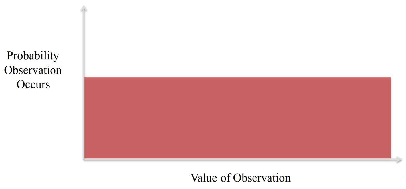
Uniform Distribution

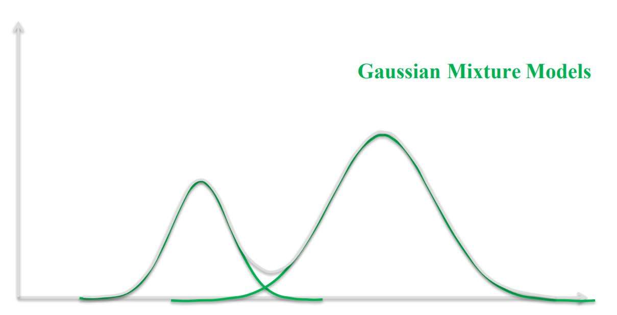
Normal (Gaussian) Distribution

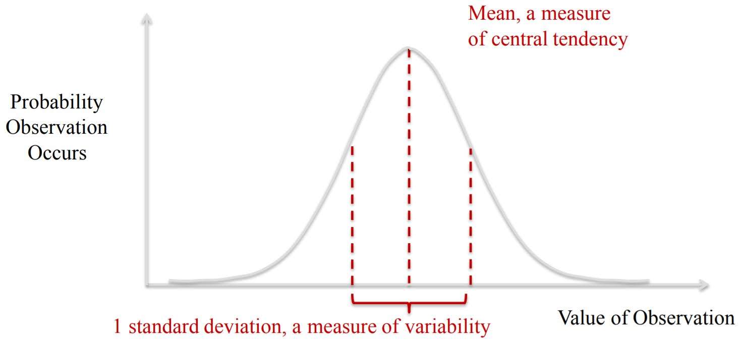
Formula for standard deviation: $\sqrt{\frac{1}{N} \sum_{i=1}^N (x_i - \overline{x})^2}$

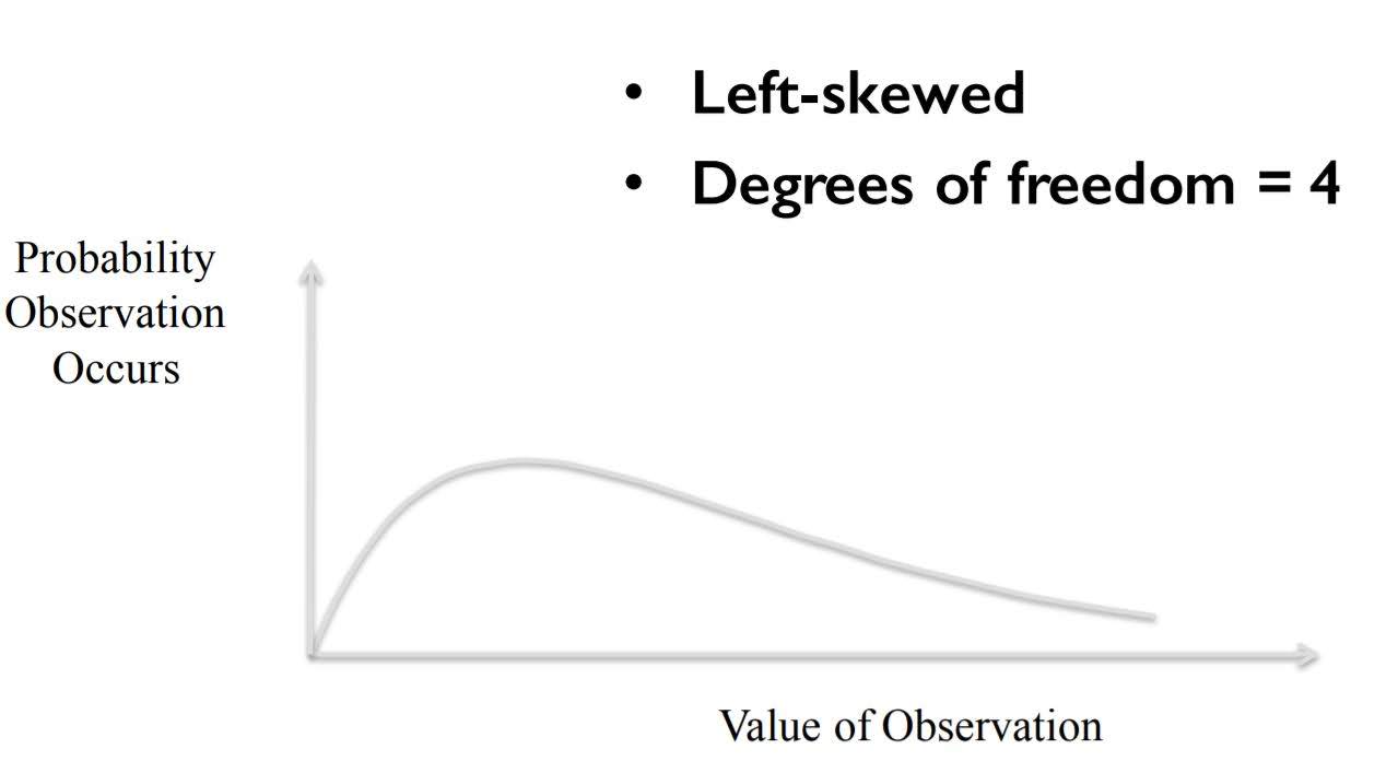
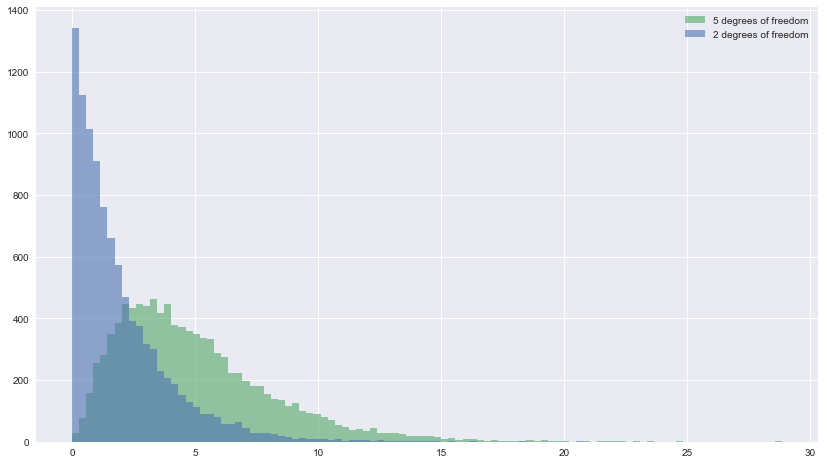
Chi Squared Distribution

Skewness & Kurtosis

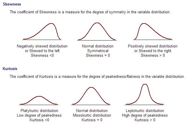
Skewness is a measure of symmetry, or more precisely, the lack of symmetry. A distribution, or data set, is symmetric if it looks the same to the left and right of the center point.
When ‘Degrees of Freedom’ gets smaller, the graph gets skewed to left.

Kurtosis is a measure of whether the data are heavy-tailed or light-tailed relative to a normal distribution. That is, data sets with high kurtosis tend to have heavy tails, or outliers. Data sets with low kurtosis tend to have light tails, or lack of outliers. A uniform distribution would be the extreme case.

Bimodal distributions

Distributions in Pandas

import pandas as pd
import numpy as np

np.random.binomial(1, 0.5)

1

# Flip 1000 coins and check number of heads. Do this 10 times.
np.random.binomial(1000, 0.5, 10)

array([502, 511, 516, 494, 527, 512, 529, 521, 495, 487])

# sample a number from uniform distribution between 0 and 1
np.random.uniform(0, 1)

0.2828033347414428

#sample a number from normald distribution of mean=0, std=1
np.random.normal(loc=0, scale=1)

-1.3560071953448096

distribution = np.random.normal(loc=0, scale=1, size=1000)
distribution.std()

0.9831044712693359

import scipy.stats as stats
stats.kurtosis(distribution)

0.025384635432275093

stats.skew(distribution)

0.055923877445990366

chi_squared_df2 = np.random.chisquare(2, size=10000)
stats.skew(chi_squared_df2)

2.0018163864318907

chi_squared_df5 = np.random.chisquare(5, size=10000)
stats.skew(chi_squared_df5)

1.3161735810606243

%matplotlib inline
import matplotlib
import matplotlib.pyplot as plt
import seaborn as sns
sns.set()

plt.figure(figsize=(14,8))
plt.hist([chi_squared_df2,chi_squared_df5], bins=100, label=['2 degrees of freedom','5 degrees of freedom'], histtype='stepfilled', alpha=0.6)
plt.legend()

<matplotlib.legend.Legend at 0x17d0be8e7f0>

Hypothesis Testing

P-value, or critical value $\alpha$ of hypothesis testing of a model shows probability that the correlation happend just on chance.
Typically in social sciences, we accept our hypothesis if p-value is less than 0.1, 0.05, or 0.01.

We will use ttest_ind.
We can use this test, if we observe two independent samples from the same or different population, e.g. exam scores of boys and girls or of two ethnic groups. The test measures whether the average (expected) value differs significantly across samples. If we observe a large p-value, for example larger than 0.05 or 0.1, then we cannot reject the null hypothesis of identical average scores. If the p-value is smaller than the threshold, e.g. 1%, 5% or 10%, then we reject the null hypothesis of equal averages.

df = pd.read_csv('grades.csv')

df.head()

	student_id	assignment1_grade	assignment1_submission	assignment2_grade	assignment2_submission	assignment3_grade	assignment3_submission	assignment4_grade	assignment4_submission	assignment5_grade	assignment5_submission	assignment6_grade	assignment6_submission
0	B73F2C11-70F0-E37D-8B10-1D20AFED50B1	92.733946	2015-11-02 06:55:34.282000000	83.030552	2015-11-09 02:22:58.938000000	67.164441	2015-11-12 08:58:33.998000000	53.011553	2015-11-16 01:21:24.663000000	47.710398	2015-11-20 13:24:59.692000000	38.168318	2015-11-22 18:31:15.934000000
1	98A0FAE0-A19A-13D2-4BB5-CFBFD94031D1	86.790821	2015-11-29 14:57:44.429000000	86.290821	2015-12-06 17:41:18.449000000	69.772657	2015-12-10 08:54:55.904000000	55.098125	2015-12-13 17:32:30.941000000	49.588313	2015-12-19 23:26:39.285000000	44.629482	2015-12-21 17:07:24.275000000
2	D0F62040-CEB0-904C-F563-2F8620916C4E	85.512541	2016-01-09 05:36:02.389000000	85.512541	2016-01-09 06:39:44.416000000	68.410033	2016-01-15 20:22:45.882000000	54.728026	2016-01-11 12:41:50.749000000	49.255224	2016-01-11 17:31:12.489000000	44.329701	2016-01-17 16:24:42.765000000
3	FFDF2B2C-F514-EF7F-6538-A6A53518E9DC	86.030665	2016-04-30 06:50:39.801000000	68.824532	2016-04-30 17:20:38.727000000	61.942079	2016-05-12 07:47:16.326000000	49.553663	2016-05-07 16:09:20.485000000	49.553663	2016-05-24 12:51:18.016000000	44.598297	2016-05-26 08:09:12.058000000
4	5ECBEEB6-F1CE-80AE-3164-E45E99473FB4	64.813800	2015-12-13 17:06:10.750000000	51.491040	2015-12-14 12:25:12.056000000	41.932832	2015-12-29 14:25:22.594000000	36.929549	2015-12-28 01:29:55.901000000	33.236594	2015-12-29 14:46:06.628000000	33.236594	2016-01-05 01:06:59.546000000

len(df)

2315

early = df[df['assignment1_submission'] <= '2015-12-31']
late = df[df['assignment1_submission'] > '2015-12-31']

early.mean()

assignment1_grade    74.972741
assignment2_grade    67.252190
assignment3_grade    61.129050
assignment4_grade    54.157620
assignment5_grade    48.634643
assignment6_grade    43.838980
dtype: float64

late.mean()

assignment1_grade    74.017429
assignment2_grade    66.370822
assignment3_grade    60.023244
assignment4_grade    54.058138
assignment5_grade    48.599402
assignment6_grade    43.844384
dtype: float64

from scipy import stats

stats.ttest_ind(early['assignment1_grade'], late['assignment1_grade'])

Ttest_indResult(statistic=1.400549944897566, pvalue=0.16148283016060577)

stats.ttest_ind(early['assignment2_grade'], late['assignment2_grade'])

Ttest_indResult(statistic=1.3239868220912567, pvalue=0.18563824610067967)

stats.ttest_ind(early['assignment3_grade'], late['assignment3_grade'])

Ttest_indResult(statistic=1.7116160037010733, pvalue=0.08710151634155668)

According to ttest_ind, mean value of assignment3 grade between early students and late students might be correlated.