Neural Style Transfer

Original Source: https://www.coursera.org/specializations/deep-learning

https://arxiv.org/abs/1508.06576

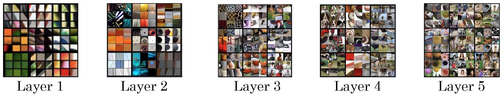
What are deep ConvNets Learning?

By finding the image patch that maximizes activation unit of layers, we can visualize what convnets are learning in each layer.

Convolutional neural network learns more complex features in deeper layers. Activations in early layers learn simple features such as straight lines, whereas activations in latter layers learn complex features such as wheels of a vehicle.

This is because early layers can only see small regions of the input image, whereas latter layers can see larger portions of the input image. (Remind how an unit of a layer only receives informations from portion of previous layer by filter.)

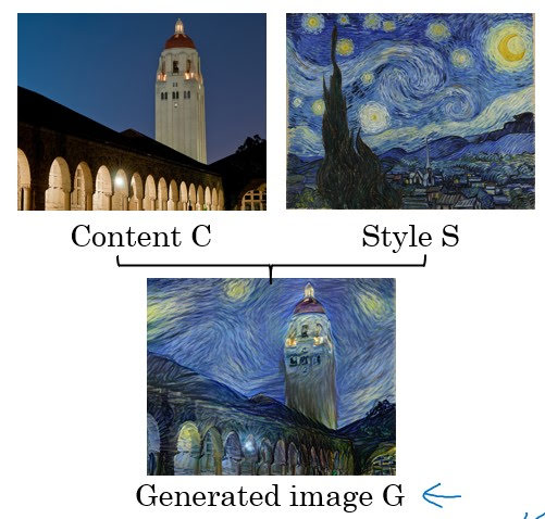
What is Neural Style Transfer?

With content C and style S, neural style transfer outputs generated image G.

Neural Style Transfer Cost Function

\[J(G) = \alpha J_{content}(C,G)+\beta J_{style}(S,G)\]

$J_{content}(C,G), J_{style}(S,G)$ computes how similar generated image is to content and style, respectively.

1. Content Cost Function

Say you use $l$th hidden layer to compute cost function. This $l$ should not be picked from too shallow layers or too deep layers. If you use hidden layer one, then it will really force your generated image to have pixel values very similar to your content image. Whereas, if you use a very deep layer, then it’s just asking, “Well, if there is a dog in your content image, then make sure there is a dog somewhere in your generated image.”

Use pre-trained ConvNet. So $a^{[l](C)}$ means an $l$ th activation unit of pre-trained convnet with input C.

\[J_{content}(C,G) = \frac{1}{2}||a^{[l](C)}-a^{[l](G)}||^2\]

If this value is small, it means that C and G are similar with respect to their activations in layer $l$. We want them to be similar, so this is a good cost function that we want to minimize.

2. Style Cost Function

We will define style as correlation between activations across channels. So if $k$ th and $k’$ th channel of layer l is highly correlated, $G_{kk’}^{[l]}$ is big.

So our ‘style matrix(gram matrix)’ of layer $l$ ($G^{[l]}$) would be of shape $c^{[l]} \times c^{[l]}$ and is computed as follows;

\[G_{kk'}^{[l]} = \sum_{i=1}^{n_H^{[l]}} \sum_{j=1}^{n_W^{[l]}} a_{ijk}^{[l]} a_{ijk'}^{[l]}\]

We want the style matrix of S and G to be similar. Thus our cost function of layer $l$ would be as follows;

\[J_{style}^{[l]} (S,G)=\frac{1}{(2n_H^{[l]} n_W^{[l]} n_C^{[l]} )^2} ‖G^{[l](S)}-G^{[l](G)} ‖_F^2\]

We divide frobenius norm by $(2n_H^{[l]} n_W^{[l]} n_C^{[l]} )^2$ just to normalize, but it doesn’t matter so much because it will be multiplied later by $\beta$ anyway.

Cost function across all layers would be the weighted sum of costs of layers.

\[J_{style} (S,G)=\sum_lλ^{[l]} J_{style}^{[l]} (S,G)\]

large $\lambda^{[l]}$ means that we want to make gram matrix of style image and generated image similar with respect to layer $l$ more.

Algorithm

Now that you know how to comput cost function, neural style transfer algorithm is simple.

1. Initiate G randomly to produce white noise image with random pixel values.
2. Compute cost $J(G)$ and use optimizing algorithm to optimize pixel values of G.