Exponentially Weighted Moving Average

Original Source: https://www.coursera.org/specializations/deep-learning

Moving average is an average of changing values.

Simple Moving Average

The simple moving average (SMA) calculates an average of the last n prices, where n represents the number of periods for which you want the average:

\[SMA = \frac{x_1 + x_2 +...+ x_n}{n}\]

Exponentially Weighted Moving Average

$v_0 = 0$

$v_t = \beta v_{t-1} + (1-\beta)x_t$

$v_t := \frac{v_t}{1-\beta^t}$ (bias correction)

$v_t$ approximates average of $x_t$ and previous $\frac{1}{1-\beta}$ $x$s. Therefore, larger the $\beta$, smoother the graph but less sensitive to change of latest $x$.

Bias Correction

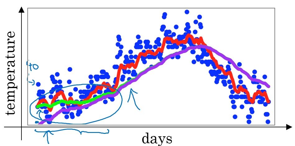
Green line is a graph after applying bias correction, and purple line is a graph without bias correction. Without bias correction, exponentially weighted moving average calculates too small value for small $t$s. Thus, smaller the $t$ is, we divide $v_t$ with smaller value($v_t := \frac{v_t}{1-\beta^t}$).

Why Use Exponentially Weighted Average?

Simple moving average is more accurate then exponentially weighted average, but why do we use exponentially weighted average?

When computing averages of a lot of variables, using simple moving average takes up a lot of memory and is computationally expensive.

But when we use exponentially weightd average, we just need one real number variable $v$ and update it when we move forward. It is both memory and computationally efficient.