GRU(Gated Recurrent Unit) and LSTM(Long Short Term Memory)

Original Source: https://www.coursera.org/specializations/deep-learning

Vanishing Gradients

Let’s say we want to train language model. With input ‘The cats, which already ate plenty of delicious biscuits’, we want the model to decide whether ‘were’ or ‘was’ will likely follow the sentence.

To let the model learn this kind of thing, when training, the loss of the layer where ‘were’ or ‘was’ appear should be backpropagated properly to the layer where ‘cats’ appear.

However, because of vanishing gradients problem, the impact of that loss to the weight-update becomes smaller as it backpropagates to ‘cats’. Thus, the relationship between ‘cats’ and ‘were’ is hardly learned by the model when these two words are far apart.

In other words, when the noun(cats) and the verb(were) are far away, the information that ‘cats’ is plural diminishes when it travels to the layer where verb appears.

There are RNN architectures that seek to solve this vanishing gradients problem in RNN. (GRU and LSTM) GRU and LSTM basically adds a ‘highway’ that far-apart units can interact directly.

GRU (Gated Recurrent Unit)

https://arxiv.org/abs/1409.1259
https://arxiv.org/abs/1412.3555

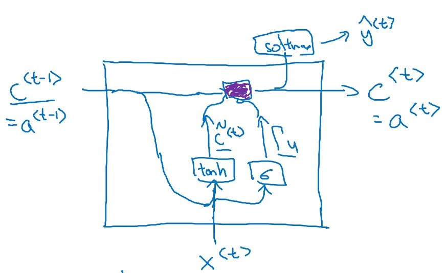
A GRU layer first computes a ‘candidate’($\tilde{c}^{<t>}$) with $c^{<t-1>}$ and $x^{<t>}$. Then, it computes ‘memory cell’ with $c^{<t-1>}$ and $\tilde{c}^{<t>}$. The memory cell becomes $a^{<t>}$.

GRU introduces a concept ‘gate’. There are two gates; gate for computing candidate(remember gate) and gate for computing memory cell(update gate).

If remember gate is 0, impact of previous activation unit to the current candidate is 0 so current candidate is computed with only $x^{<t>}$.

If update gate is 1, candidate units of that layer is directly passed to the next layer and if it is 0, activation of the previous layer is directly passed to the next layer.

1. Compute remember gate
   \(\Gamma_r = \sigma(W_r[a^{<t-1>}, x^{<t>}] + b_r)\)

2. Compute candiate for computing memory cell
   \(\tilde{c}^{<t>} = \tanh(W_c[\Gamma_r*a^{<t-1>}, x^{<t>}] + b_c)\)

3. Compute update gate
   \(\Gamma_u = \sigma(W_u[a^{<t-1>}, x^{<t>}] + b_u)\)

4. Compute memory cell
   \(\tilde{c}^{<t>} = \Gamma_u*\tilde{c}^{<t>}+(1-\Gamma_u)*c^{<t-1>}\)

5. Compute activation unit
   \(a^{<t>} = c^{<t>}\)

LSTM (Long Short Term Memory)

https://www.bioinf.jku.at/publications/older/2604.pdf

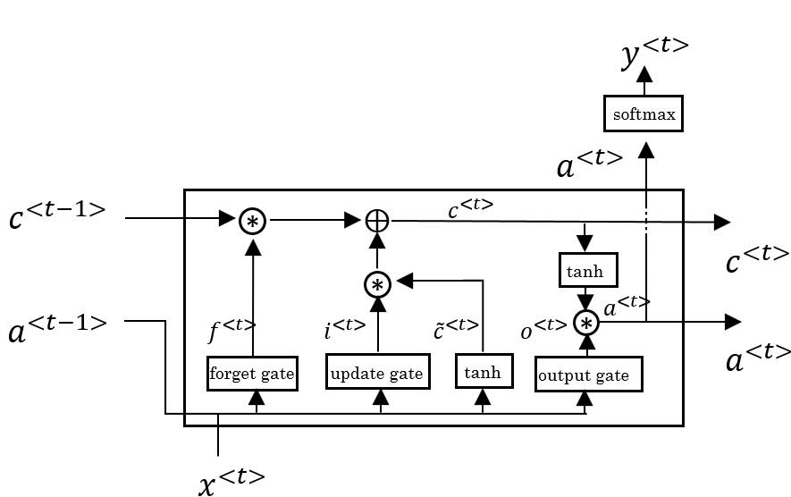
LSTM is an original version of GRU. The difference is that it has three gates.

GRU is computationally cheap, whereas LSTM is more flexible. We use LSTM as default.

1. Compute candidate
   \(\tilde{c}^{<t>} = \tanh(W_c[a^{<t-1>}, x^{<t>}] +b_c)\)

2. Compute gate for emphasizing candidate when computing memory cell (‘update gate’)
   \(\Gamma_u = \sigma(W_u[a^{<t-1>}, x^{<t>}] +b_u)\)

3. Compute gate for emphasizing previous memory cell (‘forget gate’)
   \(\Gamma_f = \sigma(W_f[a^{<t-1>}, x^{<t>}] +b_f)\)

4. Compute gate for computing activation (‘output gate’)
   \(\Gamma_o = \sigma(W_o[a^{<t-1>}, x^{<t>}] +b_o)\)

5. Compute memory cell
   \(\tilde{c}^{<t>} = \Gamma_u*\tilde{c}^{<t>}+\Gamma_f*c^{<t-1>}\)

6. Compute activation cell
   \(a^{<t>} = \Gamma_o*\tanh(c^{<t>})\)

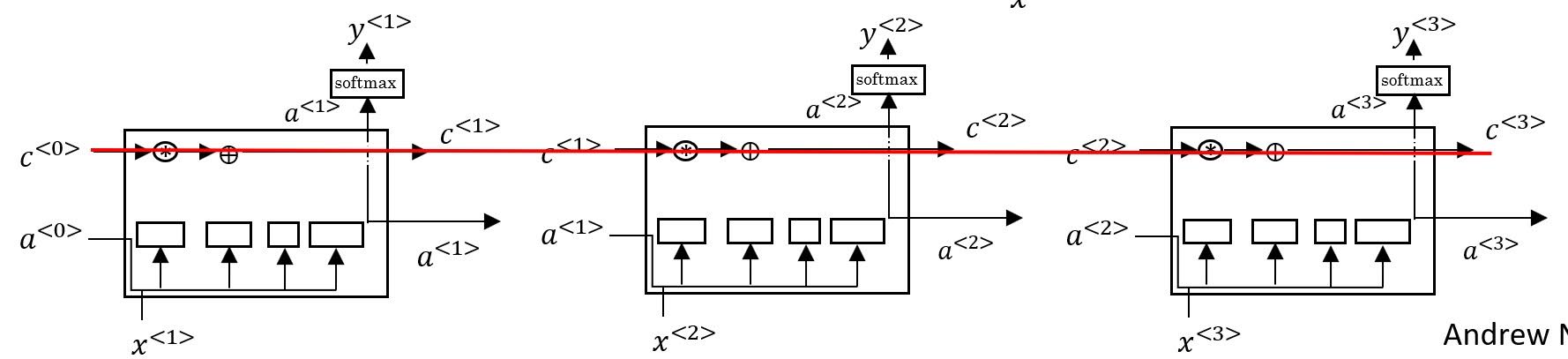
As you can see in the above image, LSTM can learn update gate to 0 and forget gate to 1 to keep memory cell intact to next layer.

Variation of LSTM: Peephole Connection

We can involve $c^{<t-1>}$ when computing gates like follows;

\[\Gamma_u = \sigma(W_u[a^{<t-1>}, x^{<t>}, c^{<t-1>}] +b_u)\] \[\Gamma_f = \sigma(W_f[a^{<t-1>}, x^{<t>}, c^{<t-1>}] +b_f)\] \[\Gamma_o = \sigma(W_o[a^{<t-1>}, x^{<t>}, c^{<t-1>}] +b_o)\]