Learning Word Embedding - Word2Vec, Negative Sampling, GloVE

Original Source: https://www.coursera.org/specializations/deep-learning

How do we learn embedding matrix?

Basically, we randomly initialize embedding matrix of shape $k \times n$ where $n$ is the size of the vocabulary and $k$ is the number of features. Then, with a large text corpus as training set, we define loss based on how frequently a ‘target’ word appears together with ‘context’ words in each example. Finally we do gradient descent(or other optimizing algorithms) to optimize embedding matrix $E$.

There are several algorithms that define loss in different ways.

Word2Vec

https://arxiv.org/abs/1301.3781

First, pick one ‘context’ word then pick one ‘target’ word that appears near the context word in training corpus. This forms one training example (also called a ‘skip-gram’). For example in a sentence ‘Yesterday, I went to school.’, you can choose to pick ‘went’ as a context and ‘school’ as a target.

Now we construct a simple neural network with input ‘context’ and label ‘target’.

For single training example, note that $\hat{y}_i$ which is the $i$ th element of our prediction $\hat{y}$, would be a probability that the target word belongs to $i$ th vocabulary. Also our label $y$ would be a one-hot representation of our target word (a vector of 0s except $t$ th element which is 1).

Let’s see how a single training example passes through our network. The parameters that we should optimize are embedding matrix $E$ and $\theta_i$ s ( $i=1,…,n$ ), which are the weight vectors associated with output $\hat{y}_i$.

\[e_c = Eo_c\]

where $o_c$ is a one-hot representation of a context word

Pass this into a layer with softmax activation.

\[\hat{y}_i = p(i|c) = \frac{exp(\theta_i^Te_c)}{\sum_{j=1}^n exp(\theta_j^Te_c)}\]

for $i=1,…,n$

\[L(\hat{y}, y) = -\sum_{i=1}^n y_i \log(\hat{y}_i)\]

Now let’s define cost that considers all of the training examples.

\[C = \frac{1}{m}\sum_{k=1}^m L\]

With this cost, we do gradient descent to optimize embedding matrix $E$ and $\theta$s.

If you pick random contexts, it is likely that most of them would be words like ‘the’ and ‘of’, so you can consider frequency of the words when picking them.

Negative Sampling

https://arxiv.org/abs/1310.4546

In Word2Vec, we’ve done a softmax classification, which is computationally expensive. But negative sampling does binary classifications.

First, pick a context word from a text corpus and a target word from near the context. This context-target pair will be a positive example. Then, pick random $k$ words from the dictionary; say $nt_1,…nt_k$. With context word $c$, these words will form pairs $(c,nt_1),…,(c,nt_k)$ . These examples will be negative examples.

Below is an example of one set of training examples and label.

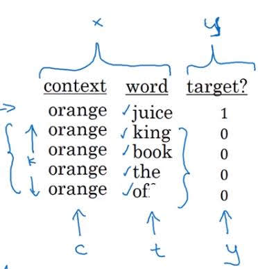
With these $k+1$ training examples, we are going to train a binary logistic classifier.

\[e_c = Eo_c\] \[\hat{y}_i = p(y=1|c,i) = \sigma(\theta_i^Te_c)\]

for $i=1,…,k+1$

We do this for many other randomly picked sets, define cost and optimize $E$ and $\theta$ s, to finally get embedding matrix $E$ .

When randomly picking a negative sample, we don’t want to randomly pick one word from corpus since then there would be too much words like ‘the’ and ‘of’, nor we want words like ‘durian’ to be picked with the same probability as words like ‘the’. We want somewhere in the middle.

Authors of the paper recommended picking with the following probability;

\[p(w_i) = \frac{f(w_i)^{3/4}}{\sum_{j=1}^n f(w_j)^{3/4}}\]

where $n$ is the size of the vocabulary and $f(w_i)$ is the frequency $i$ th word appears in corpus.

GloVE (Global Vectors for word representation)

https://www.aclweb.org/anthology/D14-1162

$X_{ij}$ : how many times target $i$ appears in context of $j$

$f(X_{ij})$ (weighting term): $f(X_{ij})=0$ if $X_{ij}=0$ . For other $X_{ij}$ s, it is manually set by us to penalize frequent words and give handicap to less frequent words.

Objective of GloVE is to minimize the following equation;

\[\min \sum_{i=1}^n \sum_{j=1}^n f(X_{ij})(\theta_i^Te_j + b_i + b_j' - log(X_{ij}))^2\]

If $X_{ij}$ is large, $\theta_i^Te_j$ needs to be large, so embeddings of $i$ and $j$ should be similar.

To compute final embedding of word $w$, we average $e_w$ and $\theta_w$ since they are perfectly symmetric while being optimized.

---

Features of embedding that have been trained by these algorithms are not interpretable by human. Nonetheless, the parallelogram map(analogy) still exists.