Neural Networks

Original Source: https://www.coursera.org/learn/machine-learning

Why Neural Networks?

We have used linear regression and logistic regression with polynomial features to represent complex relationships between input features and output. However, it was computationally inefficient, since number of features grows rapidly as we use higher polynomial degrees.

Neural networks is an alternative way and also a popular way to represent complex relationships.

What is Neural Networks?

Neural networks is basically a stack of linear regressions. More precisely, it is a stack of layers.

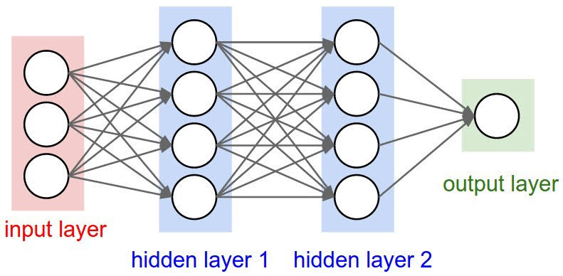
In linear and logistic regression, we had only two layers; input layer and output layer. In neural networks, we have input layer, output layer, and hidden layers.

Also, in neural networks output $Z$ of each hidden layer is fed into a function called activation function and transforms into a matrix $A$ composed of activation units which is fed as an input of next layer. This activation function is applied element-wise.

This activation function is applied to add nonlinearity to the network.

Activations

There are many possible activation functions, including sigmoid function which we’ve seen.

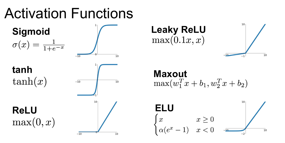
The most common one is ReLu function.

Architecture

Notations

$m$: number of training examples

$n_i$: number of features of ith layer. ($n_0$ is the number of input features)

$X$: input matrix; $m$ by $n_0$

$\Theta_i$: the weights we should optimize; $m$ by $n_i$

$Z_i$: output of linear function; $m$ by $n_i$

$A_i$: output of activation function; $m$ by $n_i$

This is an example of a neural network with two hidden layers. (In this example, $A_1$ is a matrix. It doesn’t mean anything like column vector of matrix $A$)

Input Layer

X

First Hidden Layer

\[Z_1 = X\Theta_0\] \[A_1 = g(Z_1)\]

Second Hidden Layer

\[Z_2 = A_1\Theta_1\] \[A_2 = g(Z_2)\]

Ouput Layer

for regression

\[\hat{Y}=A_2\Theta_2\]

for binary classification

\[\hat{Y}=sigmoid(A_2\Theta_2)\]

for multiclass classification

\[\hat{Y}=softmax(A_2\Theta_2)\]

Cost

For non-regularized regression and classification, cost function of neural networks is the same as the cost function we’ve seen before.

But with regularized regression and classification, the regularization term we add is slightly different since we have more $\Theta$ in nn. We add all the squares of scalar $\theta$s, multiply it with $\frac{\lambda}{2m}$ and add it to our original cost function.

Gradient Descent

To do gradient descent, we first needed to calculate partial derivatives of thetas; $\dfrac{\partial}{\partial \Theta_{i,j}^{(l)}}J(\Theta)$.

It was easy to calculate partial derivatives in logistic and linear regression. However, since there are many layers in neural networks, we have to use ‘backpropagation’ algorithm to calculate partial derivatives of thetas.

In back propagation we’re going to compute error of activation node j in layer l ($\delta_j^{(l)}$)

For the last layer, $\delta^{(L)}=a^{(L)} - y$.

To get the delta values of the layers before the last layer, we can use an equation that steps us back to left(previous) layer. \(\delta^{(l)} = ((\Theta^{(l)})^T \delta^{(l+1)})\ .*\ g'(z^{(l)})\)

We can compute our partial derivative terms by multiplying our activation values and our error values for each training example t.

\[\dfrac{\partial J(\Theta)}{\partial \Theta_{i,j}^{(l)}} = \frac{1}{m}\sum_{t=1}^m a_j^{(t)(l)} {\delta}_i^{(t)(l+1)}\]

Finally, we update thetas with gradient descent using calculated derivatives.

Random Initialization of Thetas

Initializing all theta weights to zero does not work with neural networks. If so, all nodes will update to the same value repeatedly.

Instead we can randomly initialize our weights.