Evaluation Metrics for Machine Learning Models

The recommended approach to solving machine learning problems is:

1. Start with a simple algorithm, implement it quickly, and test it early.

2. Compare cost between train and cross validation set to diagnose bias/variance.

3. Based on that result, try out implementing more models.

4. Compare evaluation metric for models to choose the best one.

It’s important to get error results as a single, numerical value. Otherwise it is difficult to assess your algorithm’s performance.

Evaluation Metrics for Regression

Mean Squared Error

We’ve used Mean Squared Error (MSE) to calculate cost of linear regression. We can use this metric as an evaluation metric too.

\[MSE = \frac{1}{m}\sum_{i=1}^m (Y_i-\hat{Y}_i)^2\]

Mean Absolute Error

\[MAE = \frac{1}{m}\sum_{i=1}^m |Y_i-\hat{Y}_i|\]

R2 Score (Coefficient of determination)

\[R^{2}=1-{\frac {\color {blue}{SS_{\text{res}}}}{\color {red}{SS_{\text{tot}}}}}\]

The better the linear regression (on the right) fits the data in comparison to the simple average (on the left graph), the closer the value of $R^{2}$ is to 1. The areas of the blue squares represent the squared residuals with respect to the linear regression. The areas of the red squares represent the squared residuals with respect to the average value.

Evaluation Metrics for Classification

Cross Entropy Loss

We’ve used cross entropy loss to calculate cost logistic regression. We can use this metric as an evaluation metric too.

\[C=-\frac{1}{m}\sum_{i=1}^m[(Y_i\cdot\log(\hat{Y_i}))+(1-Y_i)\cdot\log(1-\hat{Y_i})]\]

Accuracy

This is the basic evaluation metric for classification.

\(ACC = \frac{m_c}{m}\) where $m_c$ is the number of correctly predicted instances.

Evaluation Metrics for Skewed Classes

It is sometimes difficult to tell whether a reduction in error is actually an improvement of the algorithm.

For example: In predicting a cancer diagnoses where 0.5% of the examples have cancer, we find our learning algorithm has a 1% error. However, if we were to simply classify every single example as a 0, then our error would reduce to 0.5% even though we did not improve the algorithm.

This usually happens with skewed classes; that is, when our class is very rare in the entire data set.

Or to say it another way, when we have lot more examples from one class than from the other class.

We use below chart to make useful evaluation metrics for skewed classes.

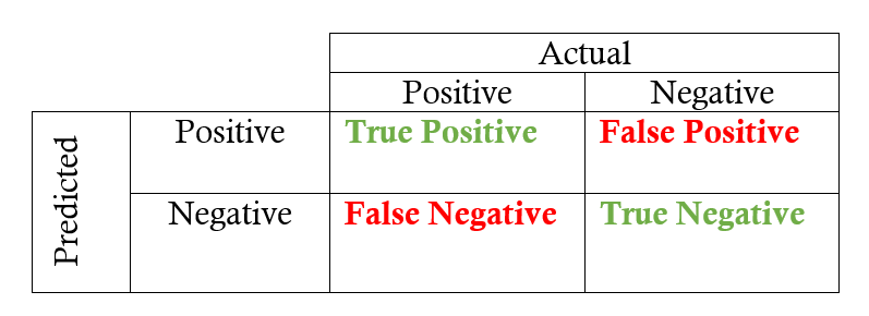
Precision

Of all patients we predicted to have cancer, what fraction actually has cancer?

\[P=\frac{TP}{TP+FP}\]

We use precision when we want confident prediction.

Recall

Of all the patients that actually have cancer, what fraction did we correctly detect as having cancer?

\[R=\frac{TP}{TP+FN}\]

We use recall when we want safe prediction.

F1 Score

There is a trade-off of precision and recall.

For example, we might want a confident prediction of two classes using logistic regression. One way is to increase our threshold:

*Predict 1 if: $h_\theta(x) \geq 0.7$ *Predict 0 if: $h_\theta(x) < 0.7$

This way, we only predict cancer if the patient has a 70% chance.

Doing this, we will have higher precision but lower recall.

If you want moderate precision and also moderate recall, you can use score that combines two; F Score.

\[F = 2\frac{PR}{P+R}\]

ROC AUC Score

A receiver operating characteristic curve, i.e., ROC curve, is a graphical plot that illustrates the diagnostic ability of a binary classifier system as its discrimination threshold is varied.

The ROC curve is created by plotting the true positive rate (TPR) against the false positive rate (FPR) at various threshold settings.

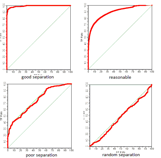
ROC AUC is the ‘Area Under the Curve’ of ROC. If the area approaches 1, it means the classifier is preforming well. If the area approaches 0.5, it means the classifier is predicting random.