Support Vector Machine (SVM) and Kernels

The Support Vector Machine (SVM) is yet another type of supervised machine learning algorithm. It is sometimes cleaner and more powerful.

Hypothesis

Hypothesis of the Support Vector Machine is not interpreted as the probability of y being 1 or 0 (as it is for the hypothesis of logistic regression). Instead, it outputs either 1 or 0. (In technical terms, it is a discriminant function.)

predict 1 when $\theta^Tx\geq0$ and 0 otherwise. ​

Cost Function

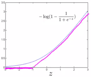
Cost function for svm is similar to binary cross entropy. The difference is that we modify terms $-\log(\frac{1}{1+e^{-z}})$ and $-\log(1-\frac{1}{1+e^{-z}})$.

We shall denote svm’s modified version of the above two terms as $\text{cost}_1(z)$ and $\text{cost}_0(z)$.

Note that $\text{cost}_1(z)$ is the cost for classifying when y=1, and $\text{cost}_0$ is the cost for classifying when y=0.

We define them as follows (where k is an arbitrary constant defining the magnitude of the slope of the line):

$z = \theta^Tx$

$\text{cost}_0(z) = \max(0, k(1+z))$

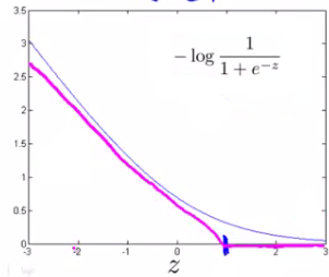
$\text{cost}_1(z) = \max(0, k(1-z))$

Also, convention dictates that we regularize using a factor C, instead of λ. Actually, C equals $\frac{1}{\lambda}$.

In conclusion, the cost function for support vector machine is as follows;

\[J(\theta) = C\sum_{i=1}^m y^{(i)} \ \text{cost}_1(\theta^Tx^{(i)}) + (1 - y^{(i)}) \ \text{cost}_0(\theta^Tx^{(i)}) + \dfrac{1}{2}\sum_{j=1}^n \Theta^2_j\]

Note that if $\theta^Tx^{(i)}\geq1$, then $cost_1(\theta^Tx^{(i)})=0$, and if $\theta^Tx^{(i)}\leq-1$, then $cost_0(\theta^Tx^{(i)})=0$.

Hyperparameter C and ‘Large Margin’

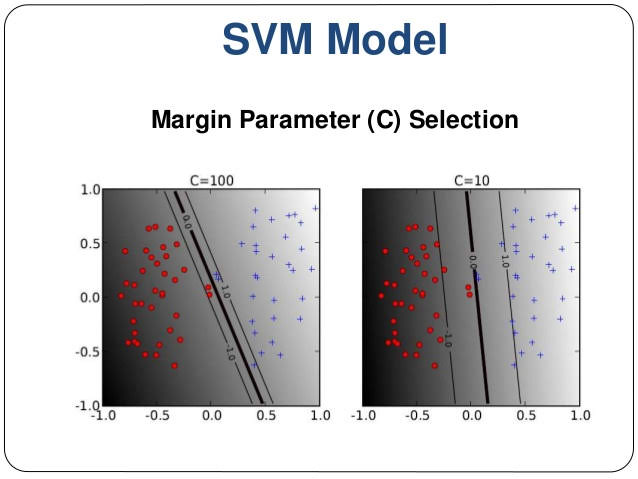
The distance of the decision boundary to the nearest example is called the margin. Since SVMs maximize this margin, it is often called a Large Margin Classifier.

If we want ‘large margin classifier’, we set C to be large.

If C is large, we should make $\sum_{i=1}^m y^{(i)} \ \text{cost}_1(\theta^Tx^{(i)}) + (1 - y^{(i)}) \ \text{cost}_0(\theta^Tx^{(i)})$ small, or 0 if possible.

We can make this term 0 if we fulfill following condition;

$\theta^Tx^{(i)}\geq1$ when $y^{(i)}=1$, and $\theta^Tx^{(i)}\leq-1$ when $y^{(i)}=0$

After fulfilling this condition, all we should do is minimize $\frac{1}{2}\sum_{j=1}^n \theta^2_j$.

If we have outlier examples that we don’t want to affect the decision boundary, then we can reduce C. When we reduce C, large margin is less likely to be achieved.

Why does minimizing $\frac{1}{2}\sum_{j=1}^n\theta_j^2$ such that $\theta^Tx^{(i)}\geq1$ when $y^{(i)}=1$, and $\theta^Tx^{(i)}\leq-1$ when $y^{(i)}=0$ makes ‘large margin’?

First we need to know two things about vectors.

1. $||v||$: The length of vector (the length of a line on a graph from origin (0,0) to $(v_1,v_2)$. The length of vector v can be calculated with $\sqrt{v_1^2 + v_2^2}$

2. $p_{vu}$: The length of projection of vector v onto vector u. $u^Tv= p_{vu} \cdot ||u||$

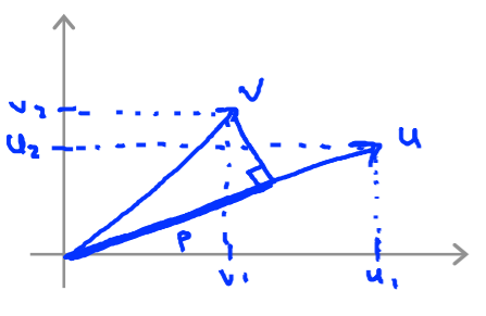
Now we know that our objective is to minimize following;

$\frac{1}{2}||\theta||^2$ such that $p_{x\theta}^{(i)}\cdot||\theta||\geq1$ when $y^{(i)}=1$, and $p_{x\theta}^{(i)}\cdot||\theta||\leq-1$ when $y^{(i)}=0$

Since $\theta$ is perpendicular to the decision boundary, $p_{x\theta}^{(i)}$ equals distance from decision boundary to $x^{(i)}$. In order to minimize $\frac{1}{2}||\theta||^2$, $p_{x\theta}^{(i)}$ needs to be large.

Kernels

Kernels allow us to make complex, non-linear classifiers using Support Vector Machines.

Support vector machine without kernel that we’ve talked about earlier is called ‘linear support vector machine’.

A kernel is a similarity function between a input vector and landmarks. We can set landmark $l^{(i)}=x^{(i)}$. We transform input vector with these kernels.

Finally, we use the outputs of these kernels as a feature vector with length m. (where m is the number of landmarks; when we use $l^{(i)}=x^{(i)}$, this value equals number of training examples.)

Each landmark $l^{(i)}$ gives us the features $f_i$. Then hypothesis becomes as follows;

\[h_\theta(x)=\theta_1f_1+\theta_2f_2+...\]

Gaussian Kernel

Gaussian kernel is one kind of kernel.

\[f_i = similarity(x, l^{(i)}) = \exp(-\dfrac{||x - l^{(i)}||^2}{2\sigma^2})\]

Note that it is efficient to do feature scaling before using the Gaussian Kernel.

Hyperparameter $\sigma^2$

With a large $\sigma^2$, the features $f_i$ vary more smoothly, causing higher bias and lower variance.

With a small $\sigma^2$, the features $f_i$ vary less smoothly, causing lower bias and higher variance.

Logistic Regression vs SVM

If n is large (relative to m), then use logistic regression, or SVM without a kernel (the “linear kernel”)

If n is small and m is intermediate, then use SVM with a Gaussian Kernel

If n is small and m is large, then manually create/add more features, then use logistic regression or SVM without a kernel.