Anomaly Detection and Gaussian Distribution

Original Source: https://www.coursera.org/learn/machine-learning

What is Anomaly Detection?

From our training examples we define a model $p(x)$ which is the probability the given instance is not anomalous.

We also use a threshold epsilon $\epsilon$ as a dividing line so we can say which examples are anomalous and which are not. If our anomaly detector is flagging too many anomalous examples, then we need to decrease our threshold $\epsilon$.

Gaussian Distribution

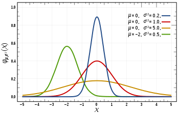
The Gaussian Distribution is a familiar bell-shaped curve that can be described by a function $\mathcal{N}(\mu,\sigma^2)$

Let x∈ℝ. If the probability distribution of $x$ is Gaussian with mean μ, variance $\sigma^2$, then $x \sim \mathcal{N}(\mu, \sigma^2)$

The little ∼ or ‘tilde’ can be read as “distributed as.”

The Gaussian Distribution is parameterized by a mean and a variance.

Mu, or μ, describes the center of the curve, called the mean. The width of the curve is described by sigma, or σ, called the standard deviation.

The full function is as follows:

\[p(x;\mu,\sigma^2) = \dfrac{1}{\sigma\sqrt{(2\pi)}}exp(-\dfrac{1}{2}(\dfrac{x - \mu}{\sigma})^2)\]

We can estimate the parameter μ from a given dataset by simply taking the average of all the examples:

\[\mu = \dfrac{1}{m}\displaystyle \sum_{i=1}^m x^{(i)}\]

We can estimate the other parameter, $\sigma^2$, with our familiar squared error formula:

\[\sigma^2 = \dfrac{1}{m}\displaystyle \sum_{i=1}^m(x^{(i)} - \mu)^2\]

Anomaly Detection Algorithm

First, calculate $\mu$ and $\sigma^2$ with the training data.

Then, given a new example $x$, compute $p(x)$.

\[p(x) = \prod^n_{j=1} p(x_j;\mu_j,\sigma_j^2)\]

Choose $\epsilon$ and predict anomaly if $p(x)<\epsilon$

Workflow

If we have 10000 good engines, 20 anomalous engines as dataset, here is the workflow of applying anomaly detection.

1. Divide examples into training set, CV set, test set.
   Training set: 6000 good engines
   CV set: 2000 good engines(y=0), 10 anomalous engines(y=1)
   Test set: 2000 good engines, 10 anomalous engines

2. Fit model p(x) on training set.

3. With cross validation example x, predict ‘y=1 if $p(x)<epsilon$, y=0 otherwise’.

4. Evaluate algorithm by F1-score, precision, recall, etc.

5. Change epsilon then evaluate again. Choose epsilon which maximizes evaluation metric.

Tips

We use supervised learning when there are enough positive examples to get a sense of what new positive examples look like. If we have a very small number of positive examples, we use anomaly detection.

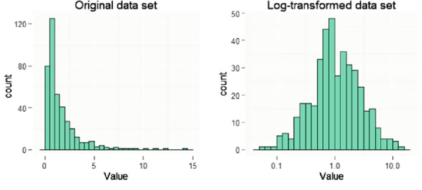
We can check that our features are gaussian by plotting a histogram of our data and checking for the bell-shaped curve.

Some transforms we can try on an example feature x that does not have the bell-shaped curve are:

• log(x)
• log(x+1)
• log(x+c) for some constant
• $\sqrt{x}$
• $x^{1/3}$