Univariate Linear Regression

Original Source: https://www.coursera.org/learn/machine-learning

What is Univariate Linear Regression?

It is basically a ‘linear regression with one variable’.

Univariate linear regression is used when you want to predict a single output value $y$ from a single input value $x$. We’re doing supervised learning here, so that means we already have an idea about what the input/output cause and effect should be.

The Hypothesis Function

Hypothesis function maps input $x$ to output $y$.

\[\hat{y}=h_\theta(x)=\theta_0+\theta_1x\]

Example

input x	output y
0	4
1	7
2	7
3	8

We will take random guess; $h_\theta(x)=4+x$

Cost Function

We can measure the accuracy of our hypothesis function by using a cost function. This takes an average of all the results of the hypothesis with inputs from x’s compared to the actual output y’s.

\[J(\theta_0,\theta_1)=\frac{1}{2m}\sum_{i=1}^m(\hat{y}_i-y_i)^2=\frac{1}{2m}\sum_{i=1}^m(h_\theta(x_i)-y_i)^2\]

This function is otherwise called the “Squared error function”, or “Mean squared error”.

The mean is halved $(\frac{1}{2m})$ as a convenience for the computation of the gradient descent.

Example

Our cost function of our random guessing $h_\theta(x)=4+x$:

\[J(1,4)=\frac{1}{2*4}((4-4)^2+(5-7)^2+(6-7)^2+(7-8)^2)=0.75\]

Gradient Descent

We need to find the parameters $\theta_i$ that minimize cost.

We put $\theta_0$ on the x axis and $\theta_1$ on the y axis, with the cost function on the vertical z axis. The points on our graph will be the result of the cost function using our hypothesis with those specific theta parameters.

We will know that we have succeeded when our cost function is at the very bottom of the pits in our graph, i.e. when its value is the minimum.

The way we do this is by taking the derivative (the tangential line to a function) of our cost function. The slope of the tangent is the derivative at that point and it will give us a direction to move towards. We make steps down the cost function in the direction with the steepest descent, and the size of each step is determined by the parameter $\alpha$, which is called the learning rate. If $\alpha$ is too large, gradient descent can overshoot the minimum and may even diverge.

Repeat until convergence:

\[\theta_j := \theta_j - \alpha \frac{\partial}{\partial \theta_j} J(\theta_0, \theta_1,...,\theta_j)\]

For univariate linear regression, gradient descent algorithm is as follows.

Repeat until convergence:

\[\theta_0:=\theta_0-\alpha\frac{1}{m}\sum_{i=1}^m(h_\theta(x_i)-y_i)\] \[\theta_1:=\theta_1-\alpha\frac{1}{m}\sum_{i=1}^m((h_\theta(x_i)-y_i)x_i)\]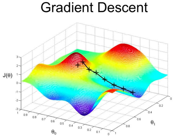

Example

One step of gradient descent of our example is as follows (when $\alpha=0.1$) \(new\theta_0 = 4-\frac{0.1}{4}((4-4)+(5-7)+(6-7)+(7-8))=4.1\) \(new\theta_1 = 1-\frac{0.1}{4}((4-4)*0+(5-7)*1+(6-7)*2+(7-8)*3)=1.175\)

Now, our hypothesis became $h_\theta(x)=1.175x+4.1$ and our cost decreased to 0.37