Logistic Regression

Original Source: https://www.coursera.org/learn/machine-learning

Notations

I will represent scalar as $x$, vector as $\vec{x}$, and matrix as $X$.

Basic

$m$: the number of training examples

$n$: the number of features

$k$: the number of output classes

$\alpha$: learning rate

$X$: an input matrix, where each row represents each training example, and each column represents each feature. Note that first column $X_1$ is a vector composed only of 1s.

$X^{(i)}$: the row vector of all the feature inputs of the ith training example

$X_j$: the column vector of all the jth feature of training examples.

$X_j^{(i)}$: value of feature j in the ith training example.

For Binary Classification

$\vec{y}$: an output column vector, where each row represents each training example.

$\vec{\theta}$: column vector of weights

$\vec{z}$: an output vector of regression step, also an input vector of sigmoid.

For Multiclass Classification

$Y$: an output matrix, where each row represents each training example, and each column represents each class.

$Z$: an output matrix of regression step, also an input matrix of softmax

$\Theta$: n by k matrix of weights

Shape of Ouput Y

Multiclass

For multiclass classification problem, output $Y^{(i)}$ will be a vector, where only one element is 1 and others 0. If mth element of that vector is 1, it means that the instance belongs to mth class.

This kind of representation is called one-hot encoding.

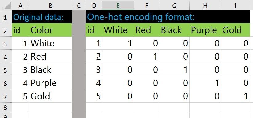
If c = number of classes and m = number of training examples, output $Y$ will be m by c matrix, where each row represents each example and column represents each class.

Binary

If the output belongs to class 0 or class 1, we do not have to make the output to be a matrix. We just need to make it a column vector $\vec{y}$, of which each row represents the probability of that training example belonging to class 1.

Hypothesis

Multiclass - Softmax

Each of our final output needs to consist only of 0 and 1.

In order to achieve it, we first apply ‘Softmax Function’ to each row of our regression output $Z$.

Softmax function transforms a vector into vector that consists values of range between 0 and 1. After applying softmax function, all the values of each row vector sums to 1.

So we can interpret ith element of the output vector of the softmax function as the probability that certain example belongs to ith class.

This is our new hypothesis function that will be applied to each row $X^{(i)}$ of the input. ($g$ is the softmax function)

\[h_\Theta(X) = g(X\Theta)\] \[g(Z^{(i)}) = \frac{e^{Z^{(i)}}}{\sum e^{Z^{(i)}}}\]

where $\sum \vec{a}$ is the sum of all elements of vector a

For each row, we assign 1 to the class that has the largest value and 0 to all the others.

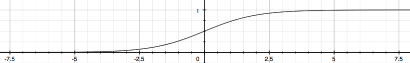
Binary - Sigmoid

Actually, sigmoid function is a binary version of softmax function. The difference is that it is applied to a scalar, not a vector.

Sigmoid function looks like this. It maps all real values to range 0~1.

This is our hypothesis for binary classfication. ($g$ is the sigmoid function)

\[h_{\vec{\theta}}(X) = g(X\vec{\theta})\] \[g(\vec{z}) = \frac{1}{1 + e^{-\vec{z}}}\]

Cost Function

Binary

\[J(\Theta)=-\frac{1}{m}\sum_{i=1}^m[(Y^{(i)}\cdot\log(h_\Theta(X^{(i)})))+((1-Y^{(i)})\cdot\log(1-h_\Theta(X^{(i)})))]\]

where $Y^{(i)}, X^{(i)}$ are ith row vector of matrix Y and X.

Why is this a ‘cost function’?

Let’s assume that $Y^{(i)}_j=1$.

If $h_\Theta(X^{(i)})_j$ is close to 1, log of it will be close to 0, so $Y_j^{(i)}\log(h_\Theta(X^{(i)})_j)$ will be close to 0. Also $1-Y_j^{(i)}$ will be 0, so $(1-Y_j^{(i)})(1-\log(h_\Theta(X^{(i)})_j))$ will also be 0. So the sum of them will be close to 0. Therefore, sum of all of those values will be close to 0, and after multiplying -1/m, it will be a positive value close to 0.

If $h_\Theta(X^{(i)})_j$ is close to 0, log of it will a lot smaller than 0, so $Y_j^{(i)}\log(h_\Theta(X^{(i)})_j)$ will be a lot smaller than 0. Therefore, even if the latter part is still 0, sum of all of those values will be very small, and after multiplying -1/m, it will be a positive value far from 0.

In conclusion, the Cost J is small when we predicted correctly, and large when we predicted wrong, so this function serves right as a cost function.

Vectorized version for binary logistic regression

\[J(\vec{\theta})=-\frac{1}{m}\Big(\vec{y}^T\log\big(h_\vec{\theta}(X)\big)+(1-\vec{y})^T\log\big(1-h_\vec{\theta}(X)\big)\Big)\]

Multiclass

\[J(\Theta)=-\frac{1}{m}\bigg(\sum_{i=1}^m \Big(Y^{(i)}\log\big(h_\Theta(X^{(i)})^T\big)\Big)\bigg)\]

Let’s say a particular example belongs to class 3. To minimize the loss of this particular example, 3rd component of $h_\Theta(X^{(i)})$ should be close to 1.

Gradient Descent

Remember that the general form of gradient descent is:

\[\begin{align*}& Repeat \; \lbrace \newline & \; \Theta_j := \Theta_j - \alpha \dfrac{\partial}{\partial \Theta_j}J(\Theta) \newline & \rbrace\end{align*}\]

We can work out the derivative part using calculus to get:

\[\begin{align*} & Repeat \; \lbrace \newline & \; \Theta_j := \Theta_j - \frac{\alpha}{m} \sum_{i=1}^m (h_\Theta(X^{(i)}) - Y^{(i)}) X_j^{(i)} \newline & \rbrace \end{align*}\]

Notice that this algorithm is identical to the one we used in linear regression.

Vectorized Version

\[\Theta := \Theta - \frac{\alpha}{m} \Big(X^T(h_\Theta(X)-Y)\Big)\]