“Representation Flow for Action Recognition” Summarized

https://arxiv.org/abs/1810.01455 (2019-8-1)

1. Optical Flow

‘Optical flow’ has been and is being used a lot for action recognition.

According to wikipedia, optical flow or optic flow is the pattern of apparent motion of objects, surfaces, and edges in a visual scene caused by the relative motion between an observer and a scene. Optical flow can also be defined as the distribution of apparent velocities of movement of brightness pattern in an image. Below is a 2D visualization of optical flow.

How do we compute optical flow?

Optical flow methods are based on the brightness consistency assumption. That is, given sequential images $I_1, I_2$, a point $x, y$ in $I_1$ is located at $x+\Delta x, y+\Delta y$ in $I_2$. It assumes small movements between frames, so this can be approximated with a Taylor series: $I_2=I_1 + \frac{\delta I}{\delta x} \Delta x + \frac{\delta I}{\delta y} \Delta y$, where $u = [\Delta x, \Delta y]$. These equations are solved for $u$ to obtain the flow, but can only be approximated due to the two unknowns.

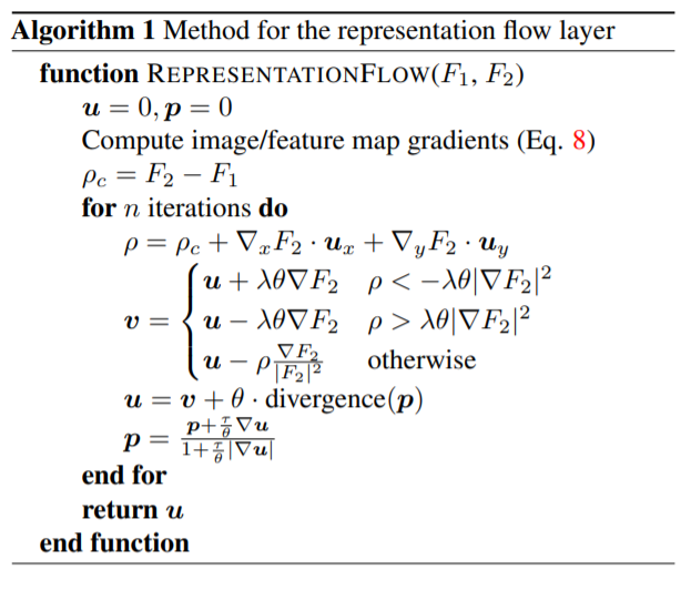
The standard, variational methods(e.g. Brox and TV-L1) estimate the flow field, $u$, using an iterative optimization method. The tensor $u \in R^{2\times W\times H}$ is the $x$ and $y$ directional flow for every location in the image. Taking two sequential images as input $I_1, I_2$, the methods first compute the gradient in both $x$ and $y$ directions: $\nabla I_2$. The initial flow is set to $u=0$. Then $\phi$ which captures the motion residual between two frames based on the current flow estimate $u$ can be computed as follows.

For efficiency, the constant part of $\phi$, $\phi_c$ is pre-computed:

\[\phi_c = I_2-\nabla_x I_2 \cdot u_x - \nabla_y I_2 \cdot u_y - I_1\]

Then, for n iterations, update $u$:

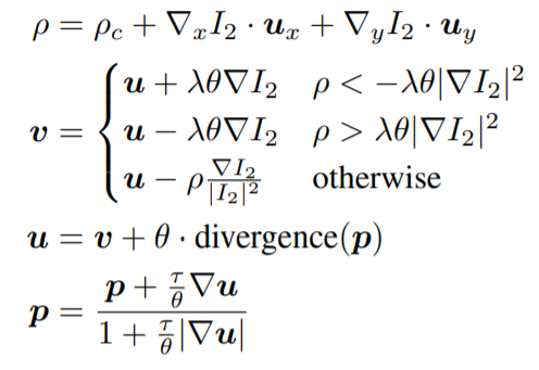
$\theta$ controls the weight of the TV-L1 regularization term, $\lambda$ controls the smoothness of the output and $T$ controls the time-step. These hyperparameters are manually set. $p$ is the dual vector fields, which are used to minimize the energy. The divergence of $p$, or backward difference, is computed as:

\[divergence(p) = p_{x,i,j} - p_{x,i-1,j} + p_{y,i,j} - p_{y,i,j-1}\]

where $p_x$ is the $x$ direction, $p_y$ is the $y$ direction, and $p$ contains all the spatial locations in the image.

The goal is to minimize the total variational energy:

\[E = |\nabla u| + \lambda |\nabla I_1*u + I_1-I_2|\]

Approaches run this iterative optimization for multiple input scales, from small to large, and use the previous flow estimate $u$ to warp $I_2$ at the larger scale, providing a coarse-to-fine optical flow estimation. These standard approaches require multiple scales and warpings to obtain a good flow estimate, taking thousands of iterations.

2. Introduction

Early, hand crafted approaches that tracked points through time were used to capture motion information.

Then, convolutional neural networks have been applied to activity recognition. Especially, two-stream networks have been very popular. They take input of a single RGB frame which captures appearance information and a stack of ‘optical flow’ frames which captures motion information. Often, the two network streams of the model are separately trained and the final predictions are averaged together. 3D spatio-temporal CNN models such as I3D also found two-stream design beneficial.

While ‘optical flow’ is known to be an important feature, flows optimized for activity recognition are often different from the true optical flow, suggesting that end-to-end learning of motion representations is beneficial. Also it is expensive to compute.

The authors propose a CNN layer called ‘representation flow’ inspired by optical flow algorithms. It learn motion representations for action recognition without having to compute optical flow separately. It is a fully-differentiable layer designed to capture ‘flow’ of any representation channels within the model. Its parameters for iterative flow optimization are learned together with other model parameters. It allows for learning of the optical flow parameters, application to any CNN feature maps (i.e. intermediate representations) and lower computational cost while maintaining performance.

3. Representation Flow Layer

‘Representation flow layer’, which the authors propose, is doing the same thing as the conventional optical flow methods, but has few differences.

1. Captures flow of any CNN feature map
2. Learns its parameters including $\theta, \lambda, T$ as well as the divergence weights
3. Only uses single scale
4. Does not perform any warping
5. Computes the flow on a CNN tensor with a smaller spatial size

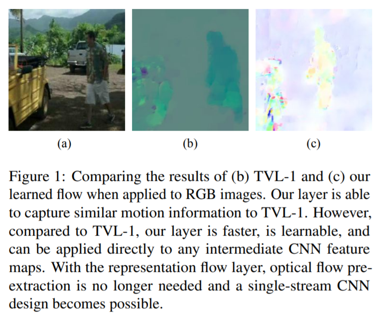
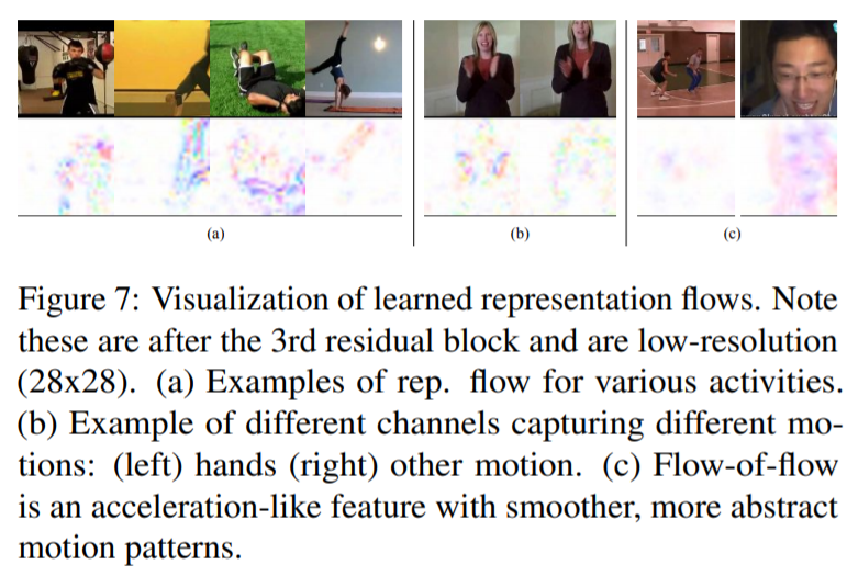
3, 4, 5 are applied to reduce compute time. The below figure compares the results of TV-L1 and learned flow presented in this paper.

Representation flow layer is applied on lower resolution CNN feature maps, instead of the RGB input. This is possible because brightness consistency assumption can similarly applied to CNN feature maps; instead of capturing pixel brightness, it captures feature value consistency.

Also, flow layer is inserted in a CNN architecture to be trained in an end-to-end fashion. The flow layer with multiple iterations could be interpreted as having a sequence of convolutional layers sharing parameters(each blue box in the below image), with each layer’s behavior dependent on its previous layer. As a result of this formulation, the layer becomes fully differentiable and allows for the learning of all optical flow parameters, enabling flow information to be optimized for its task.

The inner structure of representation flow layer is as follows.

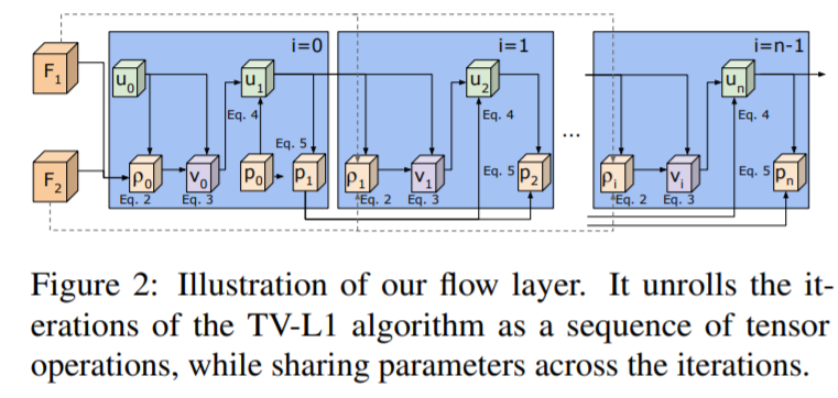
Below shows the main algorithm of representation flow layer.

4. Video-CNN Architecture

Representation flow layer is inserted between convolutional layers of video-CNN architecture. Below is the image that illustrates a video-CNN architecture with representation flow layer.

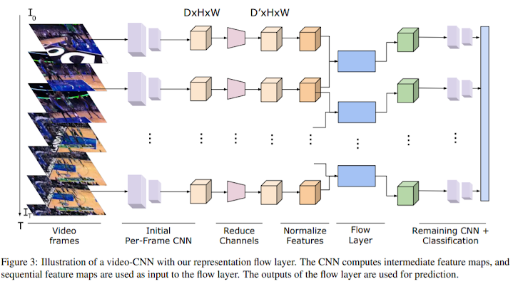
The followings are some details of the architecture.

1. Flow layer computes the flow for each channel. To save computational resource, convolutional layer is applied to reduce the number of channels.
2. For numerical stability, feature map is normalized to be in [1, 255] before inputted into the flow layer.
3. We compute the flow and stack the $x$ and $y$ flows, resulting in $2C$ channels. We apply another convolutional layer to convert from $2C$ channels to $C$ channels.
4. The CNN outputs a prediction per-timestep and these are temporally averaged to produce a probability for each class.

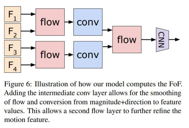
5. Flow of Flow

Applying the flow algorithm directly on two flow images means that we are tracking pixels/locations showing similar motion in two consecutive frames. In practice, this typically leads to a worse performance due to inconsistent optical flow results and non-rigid motion.

However, with representation flow layer, the flow information is ‘learned’ from the data. So it is possible to suppress such inconsistency and better abstract/represent motion by having multiple regular convolutional layers between the flow layers.

By stacking multiple representation flow layers, the model is able to capture longer temporal intervals and consider locations with motion consistency.

6. Experiments

The experiments are done with ‘Tiny-Kinetics’ dataset. For most experiments the authors used ResNet-34 with input size of 16x112x112.

1) Where to compute flow?

The authors find that computing the flow on the input provides poor performance, but there is a significant jump after even 1 layer, suggesting that computing the flow of a intermediate feature is beneficial. However, after 4 layers, the performance begins to decline as the spatial information is too abstracted/compressed.

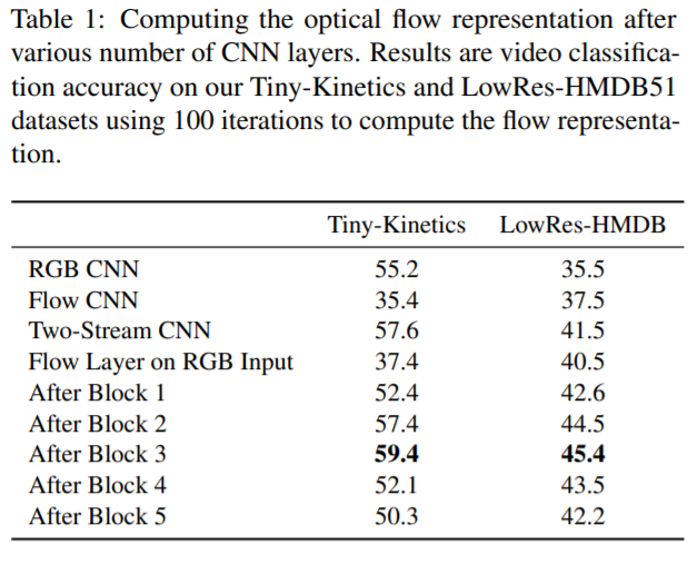
The authors apply the layer after the 3rd residual block.

2) What to learn?

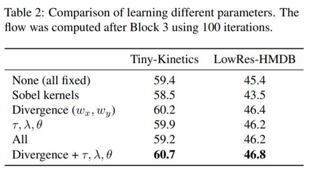
The authors find that learning the flow parameters (divergence, $\lambda, \theta, T$) is beneficial.

3) How many iterations for flow?

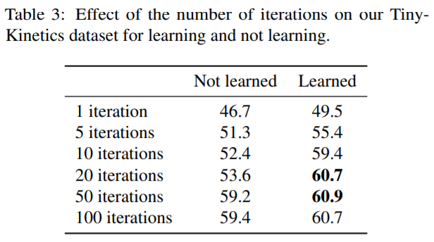
The authors used 10 or 20 iterations.

4) Two-stream fusion?

Two-stream CNNs fusing both RGB and optical flow features has been heavily studied. The authors found that fusing RGB information is very important “when computing flow directly from RGB input”. However, it is not as beneficial when computing the flow of intermediate representations as the CNN has already abstracted much appearance information away.

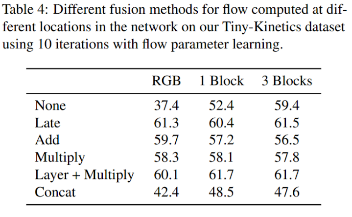
The authors didn’t use two-stream fusion in any other experiments.

5) Flow-of-flow

Applying the TV-L1 algorithm twice gives quite poor performance, as optical flow features do not really satisfy the brightness consistency assumption. Applying the representation flow layer twice performs significantly better than TV-L1 twice, but still worse than not doing so.

However, if convolutional layer is added between the first and second flow layer (flow-conv-flow; FcF), the model better learns longer-term flow representations. The authors found this performs best.

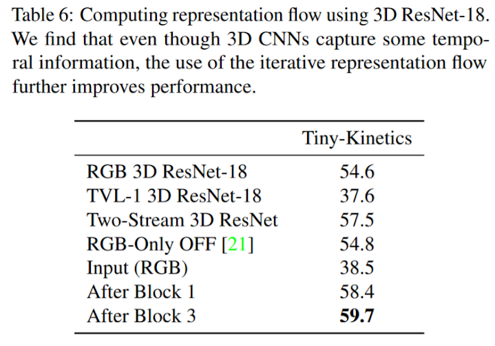
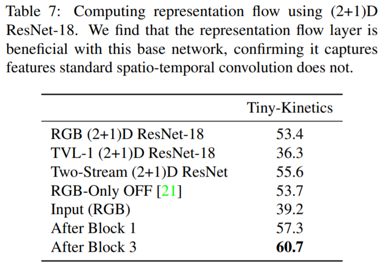
6) Flow of 3D CNN Feature

The authors find the flow layer increases performance even with 3D and (2+1)D CNNs, which already captures some temporal information.

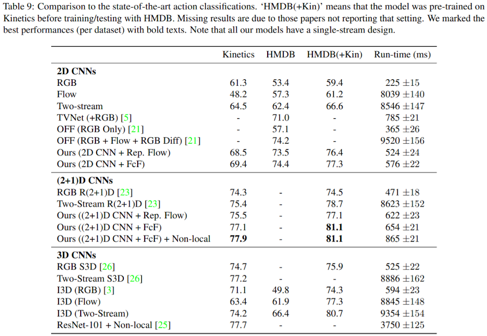
7. Comparison

1) Settings

1. Dataset: Full kinetics dataset
2. Machine: 8 V100s
3. Resolution: 32x224x224
4. Architecture: 2D ResNet-50
5. Representation flow layer after the 3rd residual block
6. Learned the hyperparameters and divergence kernels
7. 20 iterations for flow layer

2) Result