“Neural Architecture Search with Reinforcement Learning” Summarized

https://arxiv.org/abs/1611.01578 (2017-2-15)

1. Introduction

Hyperparameter optimization algorithms have been invented and used successfully before, but not with the variable-length space. The structure and connectivity of a neural network can be typically specified by a variable-length string. We used a recurrent network - the controller - to generate such string.

Training the network specified by the string on the real data will result in an accuracy on a validation set. Using this accuracy as the reward signal, we can compute the policy gradient to update the controller.

As a result, in the next iteration, the controller will give higher probabilities to archtectures that receive high accuracies. In other words, the controller will learn to improve its search over time.

The proposed Neural Architecture Search can find a novel ConvNet and RNN that is better than most human-invented architectures.

2. Controller

A ‘controller’ generates architectural hyperparameters of neural networks. To be flexible, the controller is implemented as a recurrent neural network.

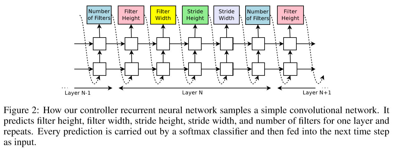
The process of generating an architecture stops if the number of layers exceeds a certain value. We increase this value as training processes.

Once the controller RNN finishes generating an architecture, a neural network with this architecture is built and trained. At convergence, the accuracy of the network on a held-out validation set is recorded.

The parameters of the controller RNN $\theta_c$ are then optimized in order to maximize the expected validation accuracy of the proposed architectures.

3. Reinforce

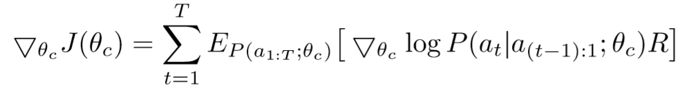
We ask our controller to maximize its expected reward, represented by $J(\theta_c) = E_{P(a_{1:T;\theta_c})}[R]$ where $a_{1:T}$ is the list of the controller’s actions, and $R$ is the reward(accuracy of the architecture).

Since the reward signal $R$ is non-differentiable, we need to use a policy gradient method to iteratively update $\theta_c$.

An empirical approximation of the above quantity is:

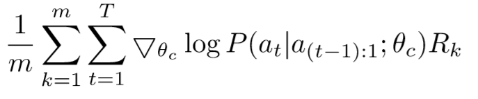
where m is the number of different architectures that the controller samples in one batch, T is the number of hyperparameters our controller has to predict, and $R_k$ is the validation accuray the k-th neural network architecture achieves after being trained on a training dataset.

The above update is an unbiased estimate for our gradient, but has a very high variance. In order to reduce the variance of this estimate we employ a baseline function:

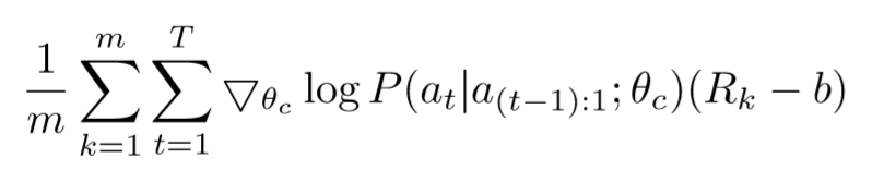
We set $b$ as an exponential moving average of the previous architecture accuracies.

4. Parallelism

We use distributed training and asynchronous parameter updates in order to speed up the learning process of the controller.

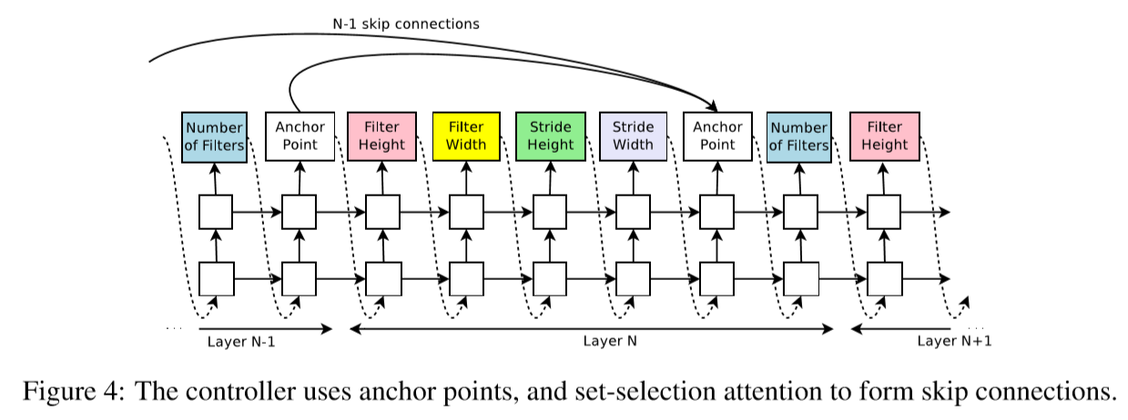
5. Skip Connections

To introduce skip connections or branching layers to the search space, wes use a set-seection type attention. At layer N, we add an anchor point which has N-1 content-based sigmoids to indicate the previous layers that need to be connected.

\[P_{ji} = sigmoid(v^Ttanh(W_{prev}*h_j+W_{curr}*h_i))\]

where $P_{ji}$ is the probability that layer j is an input to layer i $h_j$ represents the hiddenstate of the controller at anchor point for the j-th layer. $W_{prev}, W_{curr}, v$ are trainable parameters.

Skip connections can cause ‘compilation failures’ when one layer is not compatible with another layer or one layer does not have any input or output. We employ 3 techniques.

1. If a layer is not connected to any input layer then the image is used as the input layer.
2. At the final layer we take all layer outputs that hvae not been connected and concatenate them before sending this final hiddenstate to the classifier.
3. If input layers to be concatenated have different sizes, we pad the small layers with zeros.

6. RNN Generation

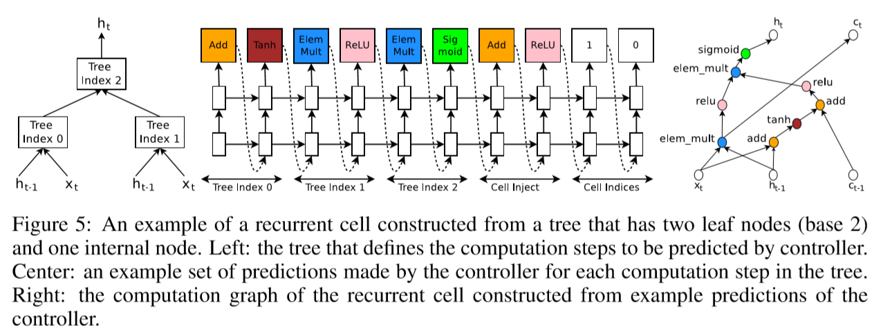
At every time step $t$, the controller needs to find a functional form for $h_t$ that takes $x_t$ and $h_{t-1}$ as inputs. (e.g. $h_t = tanh(W_1X_t+W_2h_{t-1})$ )

This computations can be generalized as a tree of steps that take $x_t$ and $h_{t-1}$ as inputs and produce $h_t$ as final output.

First we index the nodes in the tree in an order. Then the controller RNN visits each node one by one and assigns two things.

1. combination method (addition, elementwise multiplication…)
2. activation function(tanh, sigmoid…)

Inspired by LSTM, we also need $c_{t-1}$ and $c_t$ to represent the memory states. Our controller does two things.

1. It predicts combination method and activation function for injecting $c_{t-1}$. ($a_0^{new}=ReLU(a_0+c_{t-1}))$)
2. It recommends tree indices to link memory cells. The first output means tree index to where the transformed(by 1) previous hidden cell is linked. The second output means tree index to where $c_t$ is linked.

7. Cifar-10 Experiment

1) Dataset

• whitening
• upsample each image then choose a random 32x32 crop
• random horizontal flips

2) Search Space

• filter height: [1, 3, 5, 7]
• filter width: [1, 3, 5, 7]
• number of filters: [24, 36, 48, 64]

3) Controller Details

• two-layer LSTM with 35 hidden units each
• ADAM optimizer with 0.0006 lr
• weights uniformly initialized between -0.08 and 0.08
• parameter server shards S: 20 / number of replicas K: 100, number of child replicas m: 8 -> 800 networks being trained on 800 GPUs concurrently
• increase number of layers in the child networks as controller learns
• trains 12800 architectures

4) Child Model Details

• 50 epochs
• reward is the maximum validation accuracy of the last 5 epochs cubed
• Nesterov Momentum with 0.1 lr, 1e-4 weight decay, 0.9 momentum
• when the best child model is selected, we run a small grid search over learning rate, weight decay, batchnorm epsilon and what epoch to decay the learning rate and train it again to construct final model

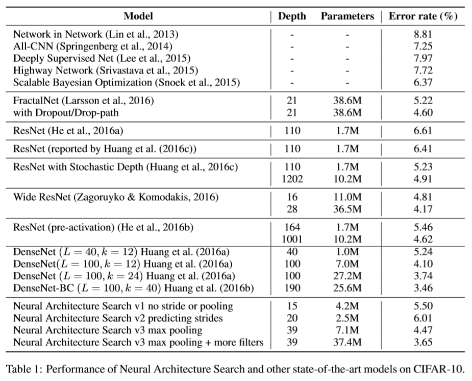
5) Result

• ask the controller to not predict stride or pooling:
  15-layer, 5.50% error rate
  has many rectangular filters
  prefers larger filters at the top layers
  has many one-step skip connections

• ask the controller to predict strides too:
  20-layer, 6.01% error rate

• allow the controller to include 2 pooling layers at layer 13 and layer 24:
  39-layer, 4.47% error rate

• add 40 more filters to each layer:
  3.65% error rate

8. Penn Treebank Experiment

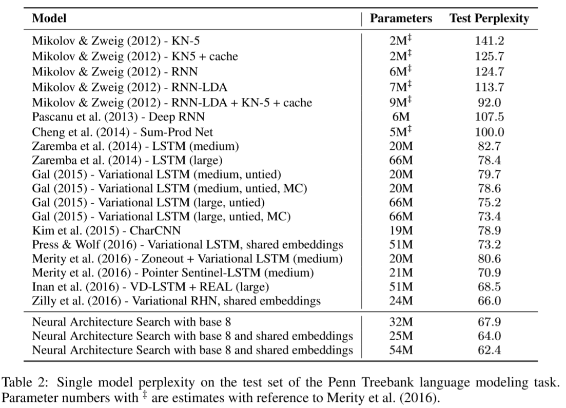
The discovered cell has many similarities to the LSTM cell in the first few steps.

The same architecture also transforms well to task such as character language modeling task on the same dataset.

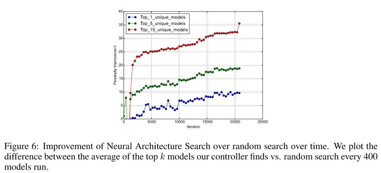
9. Control Experiment

1. Even with a bigger search space, the model can achieve somewhat comparable performance.
2. Not only the best model using policy gradient is better than the best model using random search, but also the average of top models is also much better.