“U-Net: Convolutional Networks for Biomedical Image Segmentation” Summarized

https://arxiv.org/abs/1505.04597 (2015-05-18)

1. Past Method

Ciresan et al trained a network in a sliding-window setup to predict the class label of each pixel by providing a local region (patch) around that pixel as input. But it had two drawbacks.

1. It is quite slow because the network must be run separately for each patch, and there is a lot of redundancy due to overlapping patches.
2. There is a trade-off between localization accuracy and the use of context. Larger patches require more max-pooling layers that reduce the localization accuracy, while small patches allow the network to see only little context.

2. Unet Architecture

Unet, also called “fully convolutional network” is named after its U-shaped architecture. It solves the past method’s drawbacks.

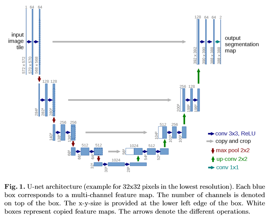
The architecture consists of a contracting path (left) and an expansive path (right).

1. Contracting Path

The contracting path consists of repeated application of the following.

1. 3x3 unpadded convolution
2. ReLU
3. 3x3 unpadded convolution
4. ReLU
5. 2x2 max pooling with stride 2 that doubles the number of feature channels

2. Expansive Path

The expansive path consists of repeated application of the following.

1. 2x2 up-convolution that halves the number of feature channels
2. concatenation with the correspondingly cropped feature map from the contracting path
3. 3x3 unpadded convolution
4. ReLU
5. 3x3 unpadded convolution
6. ReLU

At the final layer, a 1x1 convolution is used to map each 64 component feature vector to the desired number of classes.

3. Up-Convolution

Referenced https://medium.com/activating-robotic-minds/up-sampling-with-transposed-convolution-9ae4f2df52d0 .

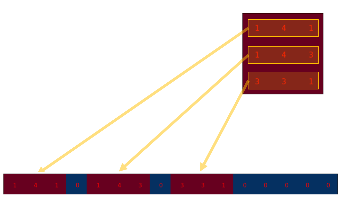
A normal convolution can also be expressed as a input multiplied with a ‘convolution matrix’ that is constructed using convolution filter. Correspondingly, transposed ‘convolution matrix’ can reverse the convolution process. We call this transposed convolution or up-convolution.

Below image describes how the first row of ‘convolution matrix’ is constructed from the convolution filter.

Then, we flatten the input and do matrix multiplication with the crafted convolution matrix to yield a vector.

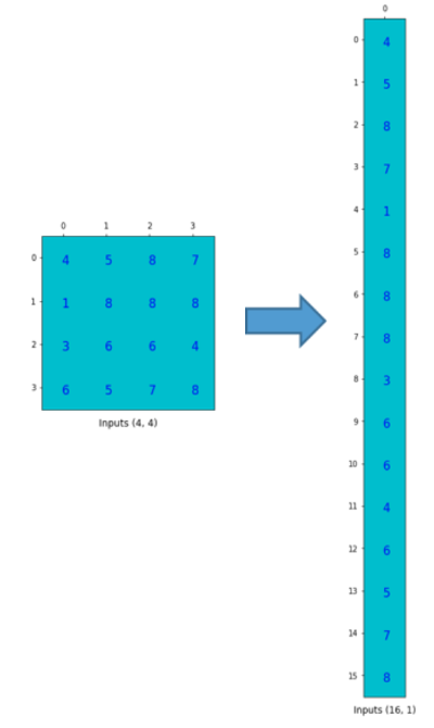
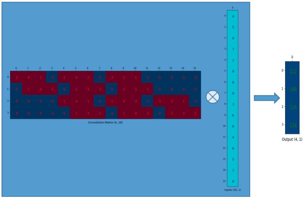
Finally we can reshape the vector to get the final output(shape of 2x2 in this case) of the operation.

Similarly, if we transpose the convolution matrix layout and do matrix multiplication with the flattened input, we can get the flattened version of the output tensor.

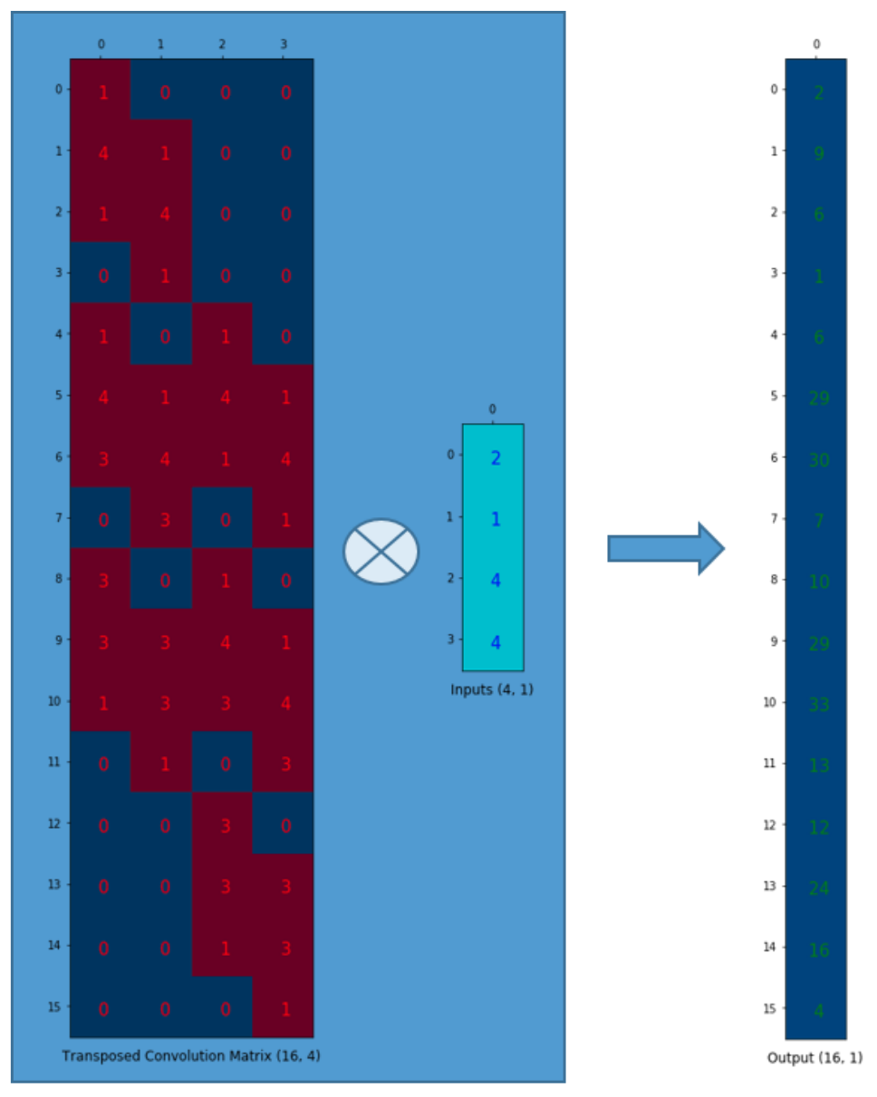
Note that the actual weight values in the matrix does not have to come from the original convolution matrix. What’s important is that the weight layout is transposed from that of the convolution matrix.

4. Overlap-Tile Strategy

Unet does not have any fully connected layers and only uses the valid part of each convolution. This allows the seamless segmentation of arbitrarily large images by an ‘overlap-tile’ strategy.

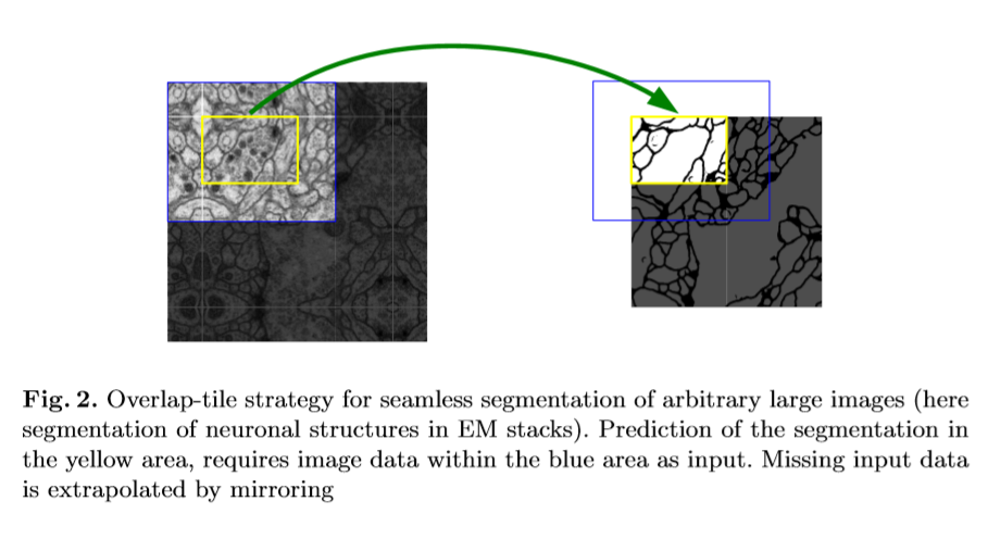
This tiling strategy is important to apply the network to large images, since otherwise the resolution would be limited by the GPU memory.

5. Loss Function

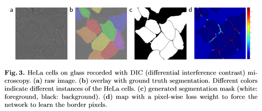
The loss function of Unet is computed by a weighted pixel-wise cross entropy.

\[L = \sum_{x\in\Omega}w(x)log(p_{l(x)}(x))\]

where $p_{l(x)}(x)$ is a softmax of a particular pixel’s true label.

We pre-compute the weight map $w(x)$ for each ground truth segmentation to

1. compensate the different frequency of pixels from a certain class in the training data set
2. force the network to learn the small separation borders that we introduce between touching cells

\[w(x) = w_c(x) + w_0 exp(-\frac{(d_1(x)+d_2(x))^2}{2\sigma^2})\]

where $w_c$ is the weight map to balance the class frequencies, $d_1$ denotes the distance to the border of the nearest cell, and $d_2$ denotes the distance to the border of the second nearest cell. The authors set $w_0=10$ and $\sigma \approx 5$ .

6. Training Details

• Initial weights are drawn from a Gaussian distribution with a standard deviation of $\sqrt{2/N}$ , where $N$ denotes the number of incoming nodes of one neuron.
• Due to the unpadded convolutions, the output image is smaller than the input by a constant border width. To minimize this overhead and make maximum use of the GPU memory, the authors favor large input tiles over a large batch size. Accordingly they used a high momentum (0.99) to weigh a large number previously seen training samples when optimizing.
• Data Augmentation: shift, rotation, gray value, particularly deformations

7. Experiment Results

1. EM segmentation challenge

2. ISBI Cell tracking challenge