“Attention Is All You Need” Summarized

https://arxiv.org/abs/1706.03762 (2017-12-6)

I would recommend you to read the amazing illustrated transformer article to understand this paper, rather than my post.

1. Background

Recurrent neural networks (RNN), long short-term memory (LSTM), and gated recurrent neural networks (GRU), have been the state of the art for sequences modeling and transduction problems such as language modeling and machine translation.

However sequential nature of these recurrent models inherently precludes parallelization within training examples, which becomes critical at longer sequence lengths, as memory constraints limit batching across examples. Also, they have difficulty catching dependencies between distant positions.

Approaches that used convolutional neural networks as basic building block were able to reduce sequential computation, but were still having difficulties with learning dependencies between distant positions.

Attention mechanisms, especially self-attention which relates different positions of a single sequence, allowed modeling of dependencies without regard to their distance in the input or output sequences, but were used in conjunction with a recurrent network.

The authors propose the Transformer, a model architecture which relies entirely on an attention mechanism to draw global dependencies between input and output. It allows for significantly more parallelization and can reach a new state of the art in translation quality.

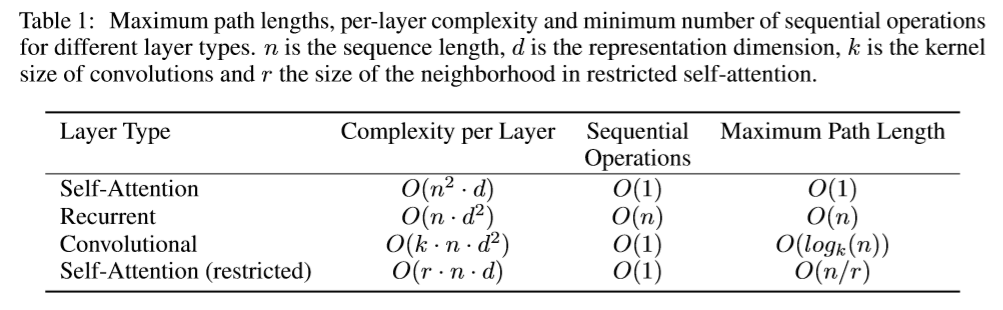
Below is a table comparing different models’ compute complexity and maximum path length between two positions.

Now let’s talk about model architecture

2. Traditional Encoder-Decoder

Most competitive neural sequence transduction models have an ‘encoder-decoder’ structure. The encoder maps an input sequence of symbol representations to a sequence of continuous ‘encoded’ representations. Given encoded representations, the decoder generates an output sequence of symbols one element at a time. At each step the model is auto-regressive, consuming the previously generated symbols as additional input when generating the next.

3. Encoder and Decoder Stacks

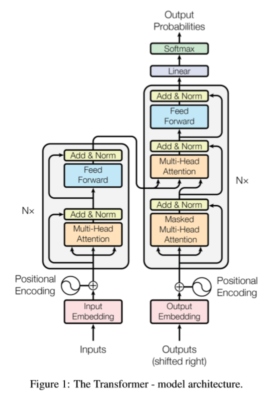
The encoder and the decoder have identical structure except that decoder has one more attention layer that uses output of the encoder.

Both are composed of a stack of 6 identical layers. Each layer has two sub-layers. The first is a multi-head self attention mechanism, and the second is a simple, position-wise fully connected feed-forward network. The authors employ a residual connection and layer normalization; $LayerNorm(x+Sublayer(x))$ . To facilitate these residual connections, all sub-layers in the model produce outputs of dimension $d_{model}=512$.

4. Scaled Dot-Product Attention

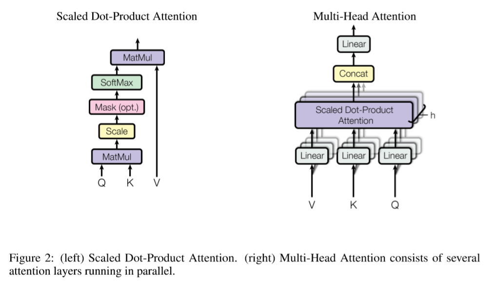
Self attention computes how a word is related to another word in a sequence. First we create 3 concepts; Q(Query), K(Key), and V(Value) by dotting input with corresponding weight matrices.

Let’s say we are processing sentence ‘I am a boy’. Think there are boxes labeled with each word. So there will be ‘I’ box, ‘am’ box, ‘a’ box and a ‘boy’ box. In each boxes, there is a document. You also have cards labeled with each word. When you are processing the word ‘am’, think that you are holding the card ‘am’ and matching it with the box labels. If it matches well, you examine the document inside thoroughly, if it does not, you just quickly see what’s inside.

Let’s think of card as a ‘Query’, box as a ‘Key’, and document inside as a ‘Value’. In self attention mechanism, these query, key, value are all vectors, and you apply a ‘compatibility function’ to calculate a scalar that represents how two match well. Then you multiply it with a value to compute the effect of a key word to a query word.

To summarize, attention is a mechanism that maps a query and a set of key-value pairs to an output. The output is computed as a weighted sum of the values, where the weight assigned to each value is computed by compatibility function of the query with the corresponding key.

The two most commonly used attention compatibility functions are additive attention and dot-product(multiplicative) attention. Additive attention computes the compatibility function using a feed-forward network with a single hidden layer, while dot-product attention just dot query and key to compute compatibility. While the two are similar in theoretical complexity, dot-product attention is much faster and more space-efficient in practice, since it can be implemented using highly optimized matrix multiplication code.

In Transformer, dot-product attention is performed as the below formula.

\[Attention(Q,K,V)=softmax(\frac{QK^T}{\sqrt{d_k}})V\]

The authors divided the term with $\sqrt{d_k}$ because they suspected that for large values of $d_k$, the dot products grow large in magnitude, pushing the softmax function into regions where it has extremely small gradients.

5. Multi-Head Attention

The authors found it beneficial to linearly project the queries, keys and values $h$ times with different, learned linear projections to $d_k, d_k, d_v$ dimensions respectively. On each of these projected versions of queries, keys and values, we then perform the attention function in parallel, yielding $h$ different $d_v$-dimensional output values. These are concatenated and once again projected, resulting in the final values.

\[head_i = Attention(QW_i^Q, KW_i^K, VW_i^V)\] \[MultiHead(Q,K,V)=Concat(head_1,...,head_h)W^O\]

Multi-head attention allows the model to jointly attend to information from different representation subspaces at different positions.

6. Applications of Attention in Transformer

1. Encoder-decoder attention

The queries come from the previous decoder layer, and the memory keys and values come from the output of the encoder. This allows every position in the decoder to attend over all positions in the input sequence.

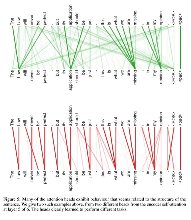
2. Encoder self-attention

All of the keys, values and queries come from the output of the previous layer. Each position in the encoder can attend to all positions in the previous layer of the encoder

3. Decoder self-attention

Each position in the decoder attend to all positions in the decoder up to and including that position. We need to prevent leftward information flow in the decoder to preserve auto-regressive property. The authors implemented this by masking out (setting to -inf) all values in the input of the softmax which correspond to illegal connections.

7. Position-wise Feed-Forward Networks

Each of the layers in encoder and decoder contains a layer with two linear transformations with a ReLU activation in between.

\[FFN(x) = max(0, xW_1+b_1)W_2+b_2\]

While the linear transformations are the same across different positions, they use different parameters from layer to layer.

8. Embeddings and Positional Encoding

Transformer uses learned embeddings to convert the encoder input tokens and decoder input tokens to vectors of dimension $d_{model}$. The same weight matrix is shared along the two embedding layers and the pre-softmax linear transformation.

In order for the model to make use of the order of the sequence, the authors added ‘positional encodings’ to the input embeddings at the bottom of the encoder and decoder stacks. There are many choices of positional encodings, learned and fixed. In Transformer, sinusoidal functions of different frequencies were used, since it produced nearly identical results as the learned version but may allow the model to extrapolate to sequence lengths longer than the ones encountered during training.

\[PE_{pos,2i}=sin(pos/10000^{2i/d_{model}})\] \[PE_{pos,2i+1}=cos(pos/10000^{2i/d_{model}})\]

It would allow the model to easily learn to attend by relative positions, since for any fixed offset $k$, $PE_{pos+k}$ can be represented as a linear function of $PE_{pos}$.

Below is a heatmap that describes positional encoding.

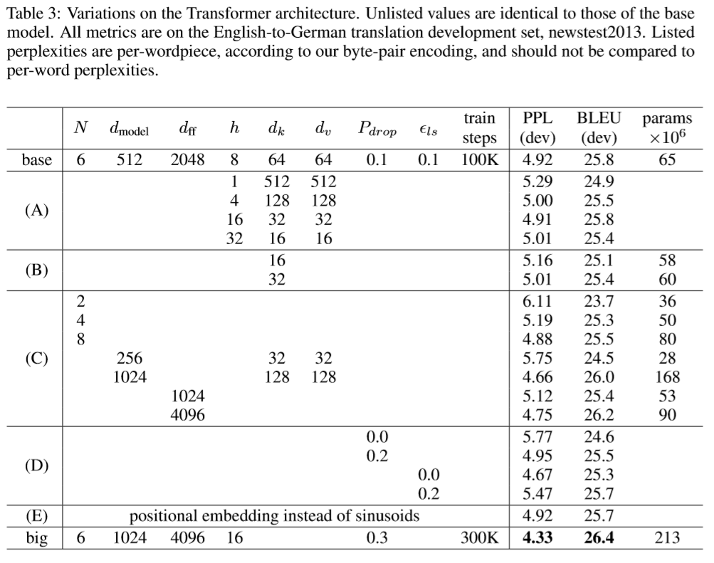
9. Training Details

Learning Rate Schedule: Increase the learning rate linearly for the first ‘warmup_steps’, and decrease it thereafter proportionally to the inverse square root of the step number.
Residual Dropout: Applied dropout to the output of each sub-layer, before it is added to the sub-layer input and normalized. Also, applied dropout to the sums of the embeddings and the positional encodings in both the encoder and decoder stacks.
Label Smoothing: of value 0.1